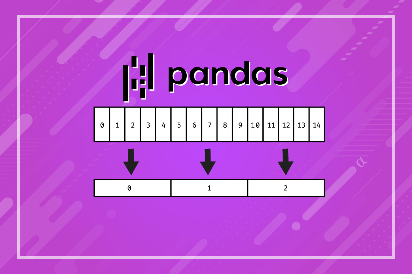
Resampling time-series data into lower-resolution intervals is easy when using Pandas and Python. The resample function, combined with the agg function, allows developers to specify how data is resampled and to what resolution.
This is useful when backtesting trading algorithms on different time periods, such as 1-minute, 5-minute, 15-minute, 4-hour, or daily periods. Aggregating time series data with pandas in this way allows multiple time resolutions to be derived from a single source. In many cases, that is the only option found in APIs or historical data archives.
Highlights
In this tutorial, we will cover how to resample an example data set containing 1-minute-resolution historical pricing data for ETH courtesy of the Binance platform. After reading this article you will learn the following:
- Use the
.read_csvfunction to load CSV data as aDataFrame, while removing un-wanted columns and dropping un-wanted rows. - Setting the index to the
datevalue and sorting the index. - Inspecting for missing dates and replacing them with NaN values.
- Defining a mapping for the
aggfunction to determine which values are to be resampled for each period and how they are to be interpreted in the process. - Resample the data into 5-minute, 15-minute, and 4-hour resolutions while.
This application of sampling would be useful in cases where one was backtesting a trading algorithm on different resolutions of data but only had a single resolution source from which to work.
TL;DR
Resampling time series data can be used to turn e.g. 1-minute resolution pricing data into e.g. 4-hour pricing data. Such resampling can be done using pandas as follows:
# Example Dataframe with 1-minute OHLC pricing data for ETH via Binance
                       symbol     open     high      low    close
date
2021-01-01 00:01:00  ETH/USDT   737.12   739.00   737.06   738.74
2021-01-01 00:02:00  ETH/USDT   738.78   738.81   737.35   737.82
2021-01-01 00:03:00  ETH/USDT   737.74   738.20   737.28   737.43
2021-01-01 00:04:00  ETH/USDT   737.38   737.80   736.80   736.89
2021-01-01 00:05:00  ETH/USDT   737.06   737.11   735.46   735.69
...                       ...      ...      ...      ...      ...
2021-12-31 23:55:00  ETH/USDT  3679.36  3679.36  3676.28  3676.65
2021-12-31 23:56:00  ETH/USDT  3676.79  3678.54  3676.32  3676.94
2021-12-31 23:57:00  ETH/USDT  3676.94  3679.01  3676.83  3677.60
2021-12-31 23:58:00  ETH/USDT  3677.56  3677.97  3672.22  3675.10
2021-12-31 23:59:00  ETH/USDT  3675.10  3678.63  3675.09  3676.23

[520542 rows x 5 columns]

# Resampling data to 4-hour intervals
df = df.resample("4H").agg({
        "open": "first",
        "high": "max",
        "low": "min",
        "close": "last"
    })

# print result
print(df)
                        open     high      low    close
date
2021-01-01 00:00:00   737.12   749.00   729.33   744.82
2021-01-01 04:00:00   744.87   747.09   734.40   737.38
2021-01-01 08:00:00   737.37   741.76   725.10   738.85
2021-01-01 12:00:00   738.85   743.33   732.12   735.39
2021-01-01 16:00:00   735.39   737.73   714.29   725.34
...                      ...      ...      ...      ...
2021-12-31 04:00:00  3742.77  3761.50  3687.00  3721.88
2021-12-31 08:00:00  3721.88  3815.00  3714.00  3780.92
2021-12-31 12:00:00  3780.92  3813.14  3773.44  3784.64
2021-12-31 16:00:00  3784.64  3788.45  3623.00  3626.27
2021-12-31 20:00:00  3626.21  3712.50  3622.29  3676.23

[2190 rows x 4 columns]
Note the agg function requires a mapping of columns and functions to define how the resample function is applied.
Quick Intro: Time Series Data & Resampling
Time series data is used across many industries to record non-stationary data. Examples include weather data, eCommerce sales data, and stock market pricing data. These are all data that have values that change over time in ways that warrant analysis.
In cases where time-series data is used, there is often a stationary “period” during which data is representative of change. For weather, the period might be hourly, daily, or monthly while other industries like securities trading records may record price history at 15-minute, 5-minute, 3-minute, or even 1-minute intervals.
Time series data is often provided in raw form, as the most granular format possible. That is; if second-resolution data is available that is the source from which minute-wise data will derive. To achieve this we use resampling which aggregates the data from multiple periods into a longer period. For example, turning 1-minute pricing history into a 15-minute pricing history.
Project Setup: Getting Price Data & Loading as DataFrame
The Pandas library for Python is a powerful data analysis package that makes working with spreadsheet data fast and efficient. Among its many functions, the resample method available to the DataFrame object will help to aggregate data. To illustrate this method’s functionality we’ll load in some minute-resolution pricing data for ETH (the transactional asset of the Ethereum network). To get started, the following steps are required:
- Have Python installed and create a new project folder with a virtual environment.
- Install pandas via
pip install pandas - Download 2021 ETH minute-resolution data from CryptoDataDownload’s Asia Binance portal (note: free account required for minute data)
With the above steps complete, we have the following project structure:
.
└── sample_project/
    └── Binance_ETHUSDT_2021_minute.csv
Inspection of the Binance_ETHUSDT_2021_minute.csv file reveals the following structure:
https://www.CryptoDataDownload.com
unix,date,symbol,open,high,low,close,Volume ETH,Volume USDT,tradecount
1640995140000,2021-12-31 23:59:00,ETH/USDT,3675.10000000,3678.63000000,3675.09000000,3676.23000000,128.71610000,473269.51792100,295
1640995080000,2021-12-31 23:58:00,ETH/USDT,3677.56000000,3677.97000000,3672.22000000,3675.10000000,129.70340000,476610.50063200,539
1640995020000,2021-12-31 23:57:00,ETH/USDT,3676.94000000,3679.01000000,3676.83000000,3677.60000000,95.80140000,352361.42737700,230
...
1609459380000,2021-01-01 00:03:00,ETH/USDT,737.74000000,738.20000000,737.28000000,737.43000000,305.98424000,225752.74457330,251
1609459320000,2021-01-01 00:02:00,ETH/USDT,738.78000000,738.81000000,737.35000000,737.82000000,418.49987000,308922.65783000,283
1609459260000,2021-01-01 00:01:00,ETH/USDT,737.12000000,739.00000000,737.06000000,738.74000000,1122.95415000,828662.13405390,643
Three important things to note here are:
- There’s a URL on the first line of the file that has to be dealt with.
- The pricing history is in descending order from newest to oldest.
- Each row has an Open, High, Low, Close, and Date value present in 1-minute increments.
With these steps complete, and a broad awareness of our data’s format, we’ll start the process of resampling with Pandas.
Loading, Inspecting, & Fixing the Data
Pandas offers the read_csv function to make loading and preprocessing CSV files easy. Using this function, the following actions are taken to load the Binance_ETHUSDT_2021_minute.csv file:
- Specify the file.
- Specify that the date should be parsed into a DateTime column.
- Specify the first row (the URL) should be skipped.
- Specify that the Date column should be used to index the data.
- Specify which columns are needed (optional)
Loading Data
All these steps can be done in one line as such:
import pandas as pd

# Load CSV data into DataFrame
df = pd.read_csv(
        'Binance_ETHUSDT_2021_minute.csv',
        skiprows=1,
        parse_dates=['date'],
        index_col=['date'],
        usecols=['date', 'open', 'high', 'low', 'close', 'symbol']
    )
At this point, we can check that our data has been ingested and converted to a DataFrame object as intended:
# print a representation of the DataFrame to the console
print(df)

# Resulting output
                       symbol     open     high      low    close
date
2021-12-31 23:59:00  ETH/USDT  3675.10  3678.63  3675.09  3676.23
2021-12-31 23:58:00  ETH/USDT  3677.56  3677.97  3672.22  3675.10
2021-12-31 23:57:00  ETH/USDT  3676.94  3679.01  3676.83  3677.60
2021-12-31 23:56:00  ETH/USDT  3676.79  3678.54  3676.32  3676.94
2021-12-31 23:55:00  ETH/USDT  3679.36  3679.36  3676.28  3676.65
...                       ...      ...      ...      ...      ...
2021-01-01 00:05:00  ETH/USDT   737.06   737.11   735.46   735.69
2021-01-01 00:04:00  ETH/USDT   737.38   737.80   736.80   736.89
2021-01-01 00:03:00  ETH/USDT   737.74   738.20   737.28   737.43
2021-01-01 00:02:00  ETH/USDT   738.78   738.81   737.35   737.82
2021-01-01 00:01:00  ETH/USDT   737.12   739.00   737.06   738.74

[520542 rows x 5 columns]
Inspecting Data
The only thing of note here is that our dates seem to be in reverse order from that which one might expect. In other words, the later dates are ordered first. This is because our DataFrame’s index is currently unsorted as seen by Pandas. We can remedy this by loading our data with the sort_index() function initially as such:
# Load data with sorted index
df = pd.read_csv(
    'Binance_ETHUSDT_2021_minute.csv',
    skiprows=1,
    parse_dates=['date'],
    index_col=['date'],
    usecols=['date', 'open', 'high', 'low', 'close', 'symbol']
).sort_index()

# View dataframe
print(df)

# Results
                       symbol     open     high      low    close
date
2021-01-01 00:01:00  ETH/USDT   737.12   739.00   737.06   738.74
2021-01-01 00:02:00  ETH/USDT   738.78   738.81   737.35   737.82
2021-01-01 00:03:00  ETH/USDT   737.74   738.20   737.28   737.43
2021-01-01 00:04:00  ETH/USDT   737.38   737.80   736.80   736.89
2021-01-01 00:05:00  ETH/USDT   737.06   737.11   735.46   735.69
...                       ...      ...      ...      ...      ...
2021-12-31 23:55:00  ETH/USDT  3679.36  3679.36  3676.28  3676.65
2021-12-31 23:56:00  ETH/USDT  3676.79  3678.54  3676.32  3676.94
2021-12-31 23:57:00  ETH/USDT  3676.94  3679.01  3676.83  3677.60
2021-12-31 23:58:00  ETH/USDT  3677.56  3677.97  3672.22  3675.10
2021-12-31 23:59:00  ETH/USDT  3675.10  3678.63  3675.09  3676.23

[520542 rows x 5 columns]
With the data sorted we can now inspect — which reveals all but the specified columns have been dropped, the date is now the index and is sorted, and there are 520542 entries representing 520,542 / 24 / 60 = 361.4875 days of 2021. That’s roughly 3.5 days’ worth of missing data — something of concern.
To check our Pandas DataFrame Timeseires for missing dates we can make use of the date_range function combined with the difference function as such:
# Get a list of missing dates and specify 1min frequency
missing = pd.date_range(df.index.min(), df.index.max(), freq='1min').difference(df.index)

# View results
print(missing)

DatetimeIndex(['2021-02-11 03:41:00', '2021-02-11 03:42:00',
               '2021-02-11 03:43:00', '2021-02-11 03:44:00',
               '2021-02-11 03:45:00', '2021-02-11 03:46:00',
               '2021-02-11 03:47:00', '2021-02-11 03:48:00',
               '2021-02-11 03:49:00', '2021-02-11 03:50:00',
               ...
               '2021-09-29 08:50:00', '2021-09-29 08:51:00',
               '2021-09-29 08:52:00', '2021-09-29 08:53:00',
               '2021-09-29 08:54:00', '2021-09-29 08:55:00',
               '2021-09-29 08:56:00', '2021-09-29 08:57:00',
               '2021-09-29 08:58:00', '2021-09-29 08:59:00'],
              dtype='datetime64[ns]', length=5057, freq=None)
That’s 5057 seconds of missing data or 5057 / 60 / 24 = 3.5118 days — roughly our suspected missing amount! With that knowledge, a little Googling turns up a press release from Binance indicating that trading on September 29th, 2021 was halted due to system maintenance. Another announcement indicates that a similar issue happened on February 11th, 2021 as well. This excuses the missing data but does nothing to help reconcile the missing entries in the DataFrame.
Dealing With Missing Data
There are many ways of dealing with missing data in Pandas. In this case, we don’t want to interpolate values or replace any values explicitly, but it would be nice to insert something into the missing trade periods to indicate missing data. In this case, we’ll use the resample function again to fill any missing values as such:
# resample data, filling the missing dates with NaN values
df = df.resample('1T').fillna(method=None)

# Print result
                       symbol     open     high      low    close
date
2021-01-01 00:01:00  ETH/USDT   737.12   739.00   737.06   738.74
2021-01-01 00:02:00  ETH/USDT   738.78   738.81   737.35   737.82
2021-01-01 00:03:00  ETH/USDT   737.74   738.20   737.28   737.43
2021-01-01 00:04:00  ETH/USDT   737.38   737.80   736.80   736.89
2021-01-01 00:05:00  ETH/USDT   737.06   737.11   735.46   735.69
...                       ...      ...      ...      ...      ...
2021-12-31 23:55:00  ETH/USDT  3679.36  3679.36  3676.28  3676.65
2021-12-31 23:56:00  ETH/USDT  3676.79  3678.54  3676.32  3676.94
2021-12-31 23:57:00  ETH/USDT  3676.94  3679.01  3676.83  3677.60
2021-12-31 23:58:00  ETH/USDT  3677.56  3677.97  3672.22  3675.10
2021-12-31 23:59:00  ETH/USDT  3675.10  3678.63  3675.09  3676.23

[525599 rows x 5 columns]

# spot check dates from 'missing' to ensure NaN values added
print(df.loc['2021-02-11 03:41:00':'2021-02-11 03:50:00'])


# Result
                    symbol  open  high  low  close
date
2021-02-11 03:41:00    NaN   NaN   NaN  NaN    NaN
2021-02-11 03:42:00    NaN   NaN   NaN  NaN    NaN
2021-02-11 03:43:00    NaN   NaN   NaN  NaN    NaN
2021-02-11 03:44:00    NaN   NaN   NaN  NaN    NaN
2021-02-11 03:45:00    NaN   NaN   NaN  NaN    NaN
2021-02-11 03:46:00    NaN   NaN   NaN  NaN    NaN
2021-02-11 03:47:00    NaN   NaN   NaN  NaN    NaN
2021-02-11 03:48:00    NaN   NaN   NaN  NaN    NaN
2021-02-11 03:49:00    NaN   NaN   NaN  NaN    NaN
2021-02-11 03:50:00    NaN   NaN   NaN  NaN    NaN
Here we see a total of 525,559 values which account for 364.99 days of 2021 — much more complete than before. Then, using values taken from our missing list, we spot-check to confirm appropriate values were added for missing data. These NaN values would conceptually be enough for a backtesting program to indicate trading had halted whereas leaving them as missing would be much less clear.
Resampling the Data
The data is in 1-minute resolution — there’s nothing that can be done about that. However, there are many cases such that 5-minute, 15-minute, hourly, 4-hour, daily, or even weekly data may need to be derived from greater resolution data. In this case, we will resample the 1-minute resolution data into a 5-minute, 4-hour, and daily resolution. The process will be the same for each:
- load the 1-minute data
- Specify a resample mapping.
- Specify a resample interval.
- Resample using the
aggfunction.
The resample mapping tells Pandas which columns should be used in our data aggregation and the functions that should be used in consideration of each. This is achieved as follows, and will be the same for each resample operation regardless of time frame:
# Defines how to aggregate pricing when downsampling OHLC
    # data into a broader time period. e.g. 1-min data -> 5 min data.
    price_mapping = {
        "open": "first",
        "high": "max",
        "low": "min",
        "close": "last"
    }
Our data have a measure for the open, high, low, and close price (OHLC Data). This represents a “candlestick” for each trading period. Below is a short explanation of each:
"open": "first": The first value for open is used for resampling."high": "max": The largest value of any sub-period is taken as the high."low": "min": The smallest value of any sub-period is taken as the low."close": "last": The last value is used as the closing value.
As an example, if 5 1-minute OHLC values were resampled into a single 5-minute OHLC, the smallest value from the 5 1-minute values would be used as the new low value and the largest value from the 5 1-minutes values would be used as the new high value. Below is how to apply this mapping via Pandas resample to each of the desired periods.
Resampling to 5-Minute Resolution
# Resample using the agg funciton to 5-minute periods
MIN_5 = df.resample("5T").agg(price_mapping)

# print result
print(MIN_5)

                        open     high      low    close
date
2021-01-01 00:00:00   737.12   739.00   736.80   736.89
2021-01-01 00:05:00   737.06   737.11   732.42   732.80
2021-01-01 00:10:00   732.87   734.08   730.03   731.14
2021-01-01 00:15:00   731.14   732.22   730.46   731.50
2021-01-01 00:20:00   731.57   731.89   729.33   731.70
...                      ...      ...      ...      ...
2021-12-31 23:35:00  3695.54  3695.65  3689.18  3689.19
2021-12-31 23:40:00  3689.20  3695.78  3689.19  3693.29
2021-12-31 23:45:00  3693.30  3693.51  3685.55  3686.59
2021-12-31 23:50:00  3686.59  3686.60  3677.81  3679.10
2021-12-31 23:55:00  3679.36  3679.36  3672.22  3676.23

[105120 rows x 4 columns]
Here we measure 105,120 rows equal to 525599 / 5 = 105,119.8 indicating our 1-minute data was successfully reduced by a fifth into 5-minute data.
Resampling to 4-Hour Resolution
# resample from 1-min to 4-hour
HR_4 = df.resample("4H").agg(price_mapping)

# print result
print(HR_4)

# results
                        open     high      low    close
date
2021-01-01 00:00:00   737.12   749.00   729.33   744.82
2021-01-01 04:00:00   744.87   747.09   734.40   737.38
2021-01-01 08:00:00   737.37   741.76   725.10   738.85
2021-01-01 12:00:00   738.85   743.33   732.12   735.39
2021-01-01 16:00:00   735.39   737.73   714.29   725.34
...                      ...      ...      ...      ...
2021-12-31 04:00:00  3742.77  3761.50  3687.00  3721.88
2021-12-31 08:00:00  3721.88  3815.00  3714.00  3780.92
2021-12-31 12:00:00  3780.92  3813.14  3773.44  3784.64
2021-12-31 16:00:00  3784.64  3788.45  3623.00  3626.27
2021-12-31 20:00:00  3626.21  3712.50  3622.29  3676.23

[2190 rows x 4 columns]
Here we measure 2190 rows equal to 525,599 / (60 * 4) = 2,189.995 indicating our conversion of 1-minute resolution into 4-hour resolution was accurate.
Resampling to Daily Resolution
# aggregate 1-minute data into daily
DAY_1 = df.resample("D").agg(price_mapping)

# Print result
print(DAY_1)

# result
               open     high      low    close
date
2021-01-01   737.12   749.00   714.29   728.91
2021-01-02   728.91   787.69   714.91   774.56
2021-01-03   774.44  1011.07   768.71   978.28
2021-01-04   978.33  1162.97   890.00  1041.43
2021-01-05  1041.45  1134.60   974.45  1099.56
...             ...      ...      ...      ...
2021-12-27  4063.57  4127.46  4031.00  4037.23
2021-12-28  4037.22  4037.23  3759.36  3792.75
2021-12-29  3792.75  3827.78  3604.20  3630.19
2021-12-30  3630.18  3769.10  3585.00  3709.27
2021-12-31  3709.27  3815.00  3622.29  3676.23

[365 rows x 4 columns]
Here we measure 365 rows that need no math to confirm accuracy.
Important Considerations
We have seen how to resample time series in Pandas down to lower-resolution samples. Throughout these examples, we’ve used the resample and agg functions to accomplish this. You may have noticed the somewhat mysterious use of 5T, 15T, and D parameters being passed to the resample function. These are TimeSeries Offset Aliases that are accurately interpreted by Pandas DataFrames.
For example, the T value represents “minutely frequency” (could also be used as min) such that 1T would be 1-minute, 3T would be 3-minute, 60T would be 60-minutes (or 1-hour). These are helpful but not always immediately clear. Knowing that T represents a single minute allows one to construct nearly any >=1 minute periodic sampling, even if the numbers become large. For example 525600T would indicate 1-year resolution.
Final Thoughts
Resampling time series data in Python is simple using the methods outlined here — using Pandas as the workhorse. The resample and agg functions make short work of what would otherwise be a tedious task. The use of the TimeSeries Offset values is a bit like magic numbers but familiar enough once one reads the documentation — or falls back to using only the T value and deriving all periods from minutes.
There are plenty of ways to get financial data — with many such sources having friendly Python APIs. More often than not, however, one is limited to a single resolution such as the minute-wise data we’ve used here as an example. In these cases, it is invaluable to have a fast and efficient means of resampling data into a period of measurement ideal for one’s application — such as trying to predict stock prices using Python or just in the calculation of single indicators such as the Average Daily Range.