Covariance is a statistical method for describing how two variables change in relationship to one another. Its measure is used to describe directional correlation such that the change in observed value for one variable is reflected by a change in another. Covariance is integral to modern statistics but often only as accompanying support within more comprehensive methods.
Covariance has applications in finance—where it can help with portfolio management by reducing risk (Bartz, 2013), machine learning—where it can help dimensionality reduction (Jang, 2007), and in clinical study design—where it can help initial stages of identifying causal relationships (Schlotz, 2008).
Highlights
- Covariance describes the relationship between two variables.
- It provides a measure of direction but not the magnitude.
- It is only used to measure the relationship between two variables and requires an equal number of serial observations for each.
- Applications include portfolio management, clinical study design, and forecasting stock prices.
- Covariance is integral to many machine learning algorithms and a key aspect of correlation analysis and regression analysis.
- NumPy, Pandas and native Python code can be used to quickly and efficiently calculate the covariance.
Introduction
Covariance is the formal mathematical expression of how one variable changes in response to another. A pair of variables are considered to have positive covariance if an increase in observed value for one variable is reflected by an increase in observed value for the other variable. Likewise, negative covariance is noted when the observed value of one variable decreases in response to the decrease in the other.
Simple covariance calculations are used in cases where two variables are being considered, such as with simple linear regression. These reflect an independent variable (predictor) and a dependent variable (response.) Covariance measures series data where an identical number of observed values are present for each variable.
Below are two charts illustrating the movements of two sets of hypothetical asset pairs.
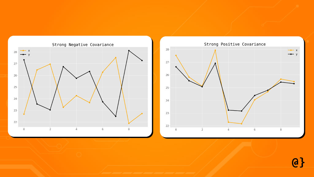
The left chart depicts assets with a strong negative covariance such as an increase in observed value for one variable is reflected by a decrease in observed value for the other. The right chart depicts two assets with strong positive covariance such that an increase in observed value for one variable is reflected by an increase in observed value for the other.
Covariance can be used to help analyze stock performance, better manage portfolio risk, and identify features for machine learning models. We’ll cover each of these applications in more detail a bit later. For now, let’s start walking through how to calculate the covariance of two series of observed values.
Calculating the Covariance
To better define covariance let’s walk through a stepwise process of its calculation. To get started, let’s define some data that will be used throughout the process:
| Observation Number |
Predictor (X) |
Response (Y) |
|---|---|---|
| 1 | 10 | 3.15 |
| 2 | 11 | 3.47 |
| 3 | 12 | 3.86 |
| 4 | 13 | 4.07 |
| 5 | 14 | 4.57 |
| 6 | 15 | 4.86 |
| 7 | 16 | 5 |
| 8 | 17 | 5.43 |
| 9 | 18 | 5.64 |
| 10 | 19 | 6.16 |
Note: The raw .csv file for this data is available for download on Github.
Step 1: Calculate the Sample Mean
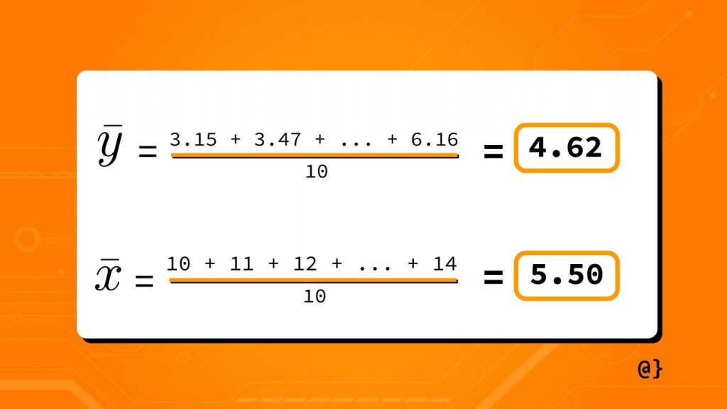
Now that we have our data we can begin the process of calculating the covariance. The first step is to calculate the sample mean for both variables in our data. The formula for this calculation is as such:
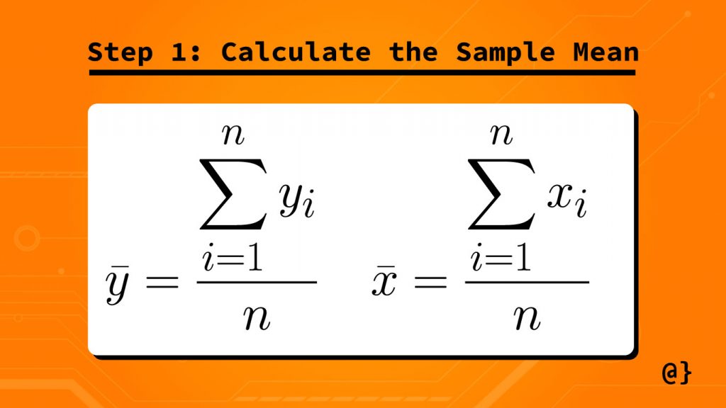
Mathematical formulae have a tendency to come off as intimidating and formal. These represent nothing more complex than saying “add all the numbers up and divide by how many are observed.” In other words—the average everyone knows and loves (arithmetic mean.) Consider the following illustration of this process:
Step 2 (optional): Calculate Signs of Sample Mean Relationships
By calculating the sign (positive vs. negative) of the relationship between each of our sample variables and their respective mean we can glean some quick insight. This step, arguably optional, describes whether the observed value of one variable might increase vs. decrease in relation to the other.
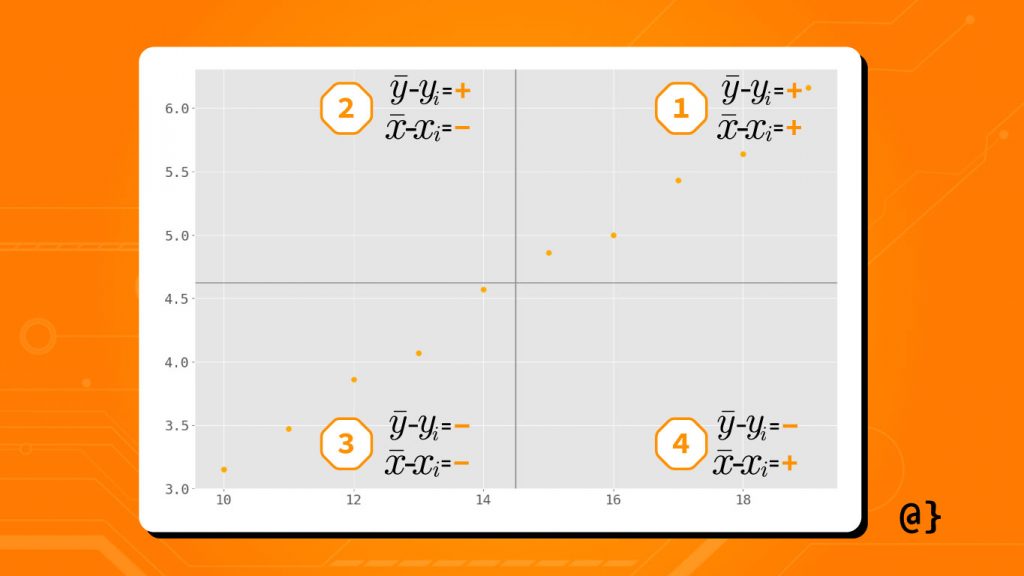
If there are more points in quadrants 1 and 3 the relationship between variables X and Y is a positive linear relationship. If there are more points in quadrants 2 and 4 the relationship between X and Y is a negative linear relationship. As a further illustration of the relationship between the sampled variable’s values and their respective sample means the following table details the resulting signs:
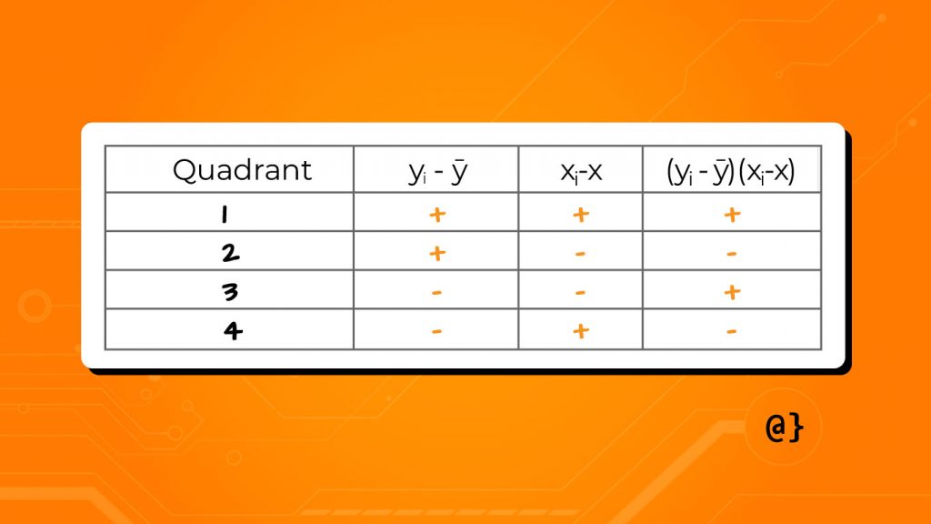
When a scatterplot of these data are not available one can use a chart similar to this one to assess whether the relationship between X and Y is positive or negative. This assessment is done by adding the values of the last column. If the value is positive, the linear relationship between X and Y positive. If the value is negative, the linear relationship between X and Y is negative. This can also be used when the scatterplot doesn’t show a clear linear relationship (low r-value.)
Step 3: Calculate the Covariance
In the above scatter plot note that more points are observed in the 1st and 3rd quadrants. This observation indicates a positive linear relationship between the values of x and y. This is supported by summing the results of the (yi – ȳ)(xi-x̄) column values which results in the positive value of ~26.61 in the case of our sample dataset. The values for this calculation can be seen in the table below:
| Observation Number |
Predictor (X) |
xi-x̄ | Response (Y) |
yi – ȳ | (yi – ȳ)(xi-x̄) |
|---|---|---|---|---|---|
| 1 | 10 | 4.5 | 3.15 | -1.471 | -6.6195 |
| 2 | 11 | 5.5 | 3.47 | -1.151 | -6.3305 |
| 3 | 12 | 6.5 | 3.86 | -0.761 | -4.9465 |
| 4 | 13 | 7.5 | 4.07 | -0.551 | -4.1325 |
| 5 | 14 | 8.5 | 4.57 | -0.051 | -0.4335 |
| 6 | 15 | 9.5 | 4.86 | 0.239 | 2.2705 |
| 7 | 16 | 10.5 | 5 | 0.379 | 3.9795 |
| 8 | 17 | 11.5 | 5.43 | 0.809 | 9.3035 |
| 9 | 18 | 12.5 | 5.64 | 1.019 | 12.7375 |
| 10 | 19 | 13.5 | 6.16 | 1.539 | 20.7765 |
Note: The data from this table is available for download on Github
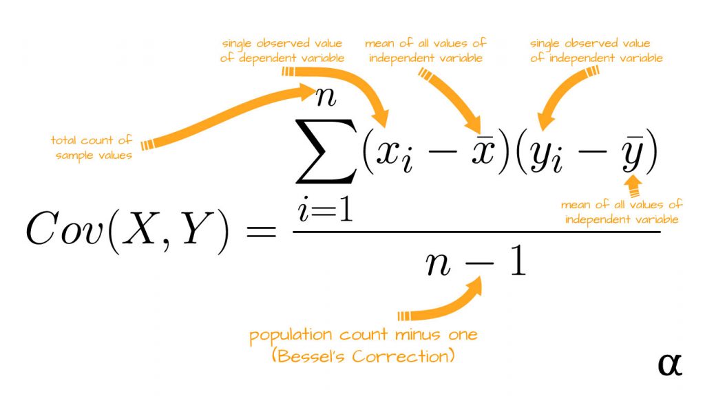
This value still needs to be standardized before it becomes useful in predicting the relationship between x and y. This is done by dividing by the total number of samples minus one—culminating in our successful execution of the covariance formula. Below is a visual depiction of which aspects of the formula for covariance these values represent.
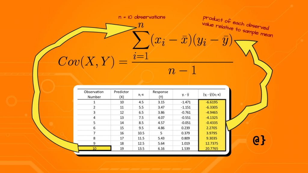
Plugging the above data and resulting calculations into the covariance formula returns a value of ~2.96—the covariance of x and y! We’ve approached this in such a painstakingly granular way solely for the thrills and for the purpose of education. In practice, covariance is calculated with more modern tools such as those available in Python. Now that we can appreciate all the hard work these tools do for us let’s consider how to set them up!
Calculating the Covariance in Python
Python can be used to calculate the covariance of two series in a number of ways. Below are several approaches to calculating the covariance in Python utilizing popular scientific libraries like NumPy and Pandas. In addition, we’ll show how to implement a covariance calculation as a custom function. Just as a quick refresher, this is our current data:
# Predictor variable series
x = [10, 11, 12, 13, 14, 15, 16, 17, 18, 19]

# Response variable series
y = [3.15, 3.47, 3.86, 4.07, 4.57, 4.86, 5, 5.43, 5.64, 6.16]
Option 1: Covariance with Pandas
Pandas offers several ways to calculate covariance. We’ll start with the simplest approach utilizing the Series.cov() method:
import pandas as pd

# Use the .cov() method to calculate
# the covariance of the variable series
cov = pd.Series(x).cov(pd.Series(y))

# Print the return value and type
print(cov, type(cov))

# Note the type is a numpy class
2.956111111111111 <class 'numpy.float64'>
The Series.cov() method is a straightforward approach when one is starting with raw data such as lists or dicts. Check out the official documentation for more information on how to specify minimum observations and degrees of freedom. Note that this method results in a type numpy.float64. This is because Pandas DataFrame, Series, and Index objects rely heavily on NumPy arrays under the hood.
Pandas also has a Dataframe.cov() method that calculates covariance which returns a covariance matrix. This type of approach is more applicable to multivariate data so we’ll skip over that for now. The NumPy method for calculating covariance will offer a sneak-peek into that data structure.
Option 2: Covariance with NumPy
The NumPy.cov() function calculates a covariance matrix for a number of variable series. It is a bit like using a sledgehammer to drive a penny nail in the case of calculating the covariance for only two variables. Nonetheless, it’s useful to be aware of:
import numpy as np

# Generate the covariance matrix
cov_matrix = np.cov(x, y)

# Print the result
print(cov_matrix)

# Results
[[9.16666667 2.95611111]
 [2.95611111 0.95956556]]

# Get the value we're interested in
cov = cov_matrix[0][1]

# Print that value + type
print(cov, type(cov))

# Results
2.956111111111111 <class 'numpy.float64'>
This method of calculating the covariance produces a matrix of values (remember we skipped that with Pandas.) We aren’t going to discuss the specifics of covariance matrices here but will note they are useful in identifying potential correlations between large numbers of variables (multivariate data.) While overkill for our example, we can still extract the covariance between x and y by indexing into the matrix (2D array).
Option 3: Custom Covariance Function
Python contains all the tools one needs to implement the covariance calculation using only built-in functions. Below is a custom implementation that first calculates the sample means, then the product of the difference of variables and their respective sample means, and returns that valued divided by the total sample size minus one:
# ensure series contain same number of elements
if len(x) != len(y):
    raise Exception("Series must be of equal length!")

# Calculate the sample means once
x_mean = sum(x) / len(x)
y_mean = sum(y) / len(y)

# Calculate the sum of the product between
# the differences of observed values and their
# respective sample means.
cov = 0.0
for xi, yi in zip(x, y):
    cov += (xi - x_mean) * (yi - y_mean)

# Divide the covariance by the
# number of samples minus 1
cov = cov / (len(x) - 1)

# Print the result
print(cov, type(cov))

# Result
2.9561111111111114 <class 'float'>
Note: This code is available as a function via Github
Examples
Its important to always remember that covariance only measures the direction and not magnitude. This limits the utility of the measure but does not negate it entirely. Covariance can help with early-stage feature selection by identifying relationships between variables in a computationally cheaper manner than full-scale correlation analysis. Below is an example of a covariance matrix to visualize the covariance between different features in a multivariate model (Zhou, 2026):

Applications
Covariance is frequently used to analyze stock prices relative to one another or between price and common indicators such as earnings reports (Ghorbani, 2020). For example, the market price of a stock tends to increase with positive earnings reports and negatively on negative earnings reports.
Covariance is utilized in the application of Modern Portfolio Theory (MPT) where it has been used to balance assets to achieve the desired level of risk for decades (Mercurio, 2020). For example, assets exhibiting negative covariance are inherently less-risky since a loss of one is likely to be offset by gains in the other. Covariance, among other statistical methods, allows MPT to assess the performance of an asset relative to its impact on the portfolio as a whole.
Covariance is also used in the Capital Asset Pricing Model (CAPM) much in the way it is utilized by MPT—to reduce risk. CAPM applies an approach known as Time-varying covariances that measure the performance of an asset relative to the rest of the portfolio over a period of time. This calculation is often made within a larger analysis such as multivariate regression (Bollerslev, 2021, ).
Review
Covariance is a fundamental tool in describing the nature of relationships in mathematical terms. We’ve seen how it can be manually calculated as well as derived from powerful modern tools like Python—either natively or via powerful scientific packages like NumPy or Pandas (or both!)
Covariance is a useful tool whether you are selecting portfolio assets to meet your risk level or selecting features in your regression model. Covariance is but one step in a larger discipline of correlation analysis and plays an integral role in the development of many highly utilized machine learning algorithms and frameworks within the most popular programming languages today.
References
- Gourlay, Neil. “Covariance Analysis And Its Applications In Psychological Research.” British Journal of Statistical Psychology, vol. 6, no. 1, 1953, pp. 25–34. Crossref, doi:10.1111/j.2044-8317.1953.tb00128.x.
- Bartz, Daniel et al. “Directional variance adjustment: bias reduction in covariance matrices based on factor analysis with an application to portfolio optimization.” PloS one vol. 8,7 e67503. 3 Jul. 2013, doi:10.1371/journal.pone.0067503
- Jang, Eunice Eunhee, and Louis Roussos. “An Investigation into the Dimensionality of TOEFL Using Conditional Covariance-Based Nonparametric Approach.” Journal of Educational Measurement, vol. 44, no. 1, 2007, pp. 1–21. Crossref, doi:10.1111/j.1745-3984.2007.00024.x.
- Schlotz, Wolff et al. “Covariance between psychological and endocrine responses to pharmacological challenge and psychosocial stress: a question of timing.” Psychosomatic medicine vol. 70,7 (2008): 787-96. doi:10.1097/PSY.0b013e3181810658
- Ghorbani, Mahsa, and Edwin K P Chong. “Stock price prediction using principal components.” PloS one vol. 15,3 e0230124. 20 Mar. 2020, doi:10.1371/journal.pone.0230124
- Bollerslev, Tim, et al. “A Capital Asset Pricing Model with Time-Varying Covariances.” Journal of Political Economy, vol. 96, no. 1, 1988, pp. 116–131. JSTOR, www.jstor.org/stable/1830713. Accessed 14 July 2021.
- “Estimating time-varying variances and covariances via nearest neighbor multivariate predictions: applications to the NYSE and the Madrid Stock Exchange Index.” Applied Economics, 41:26, 3437-3445, 2009. doi:10.1080/00036840701439371
- Zhou, Yi-Hui. “A robust covariance testing approach for high-throughput data.” arXiv: Methodology (2016): n. pag.
- Mercurio, Peter Joseph et al. “An Entropy-Based Approach to Portfolio Optimization.” Entropy (Basel, Switzerland) vol. 22,3 332. 14 Mar. 2020, doi:10.3390/e22030332


