Pandas: Select a Sub-Set Range of Dates in Time Series Data

Time Series data is used in all types of applications ranging from weather monitoring to stock trading. Pandas DataFrame objects can natively index a Time Series data and provide performant analysis.

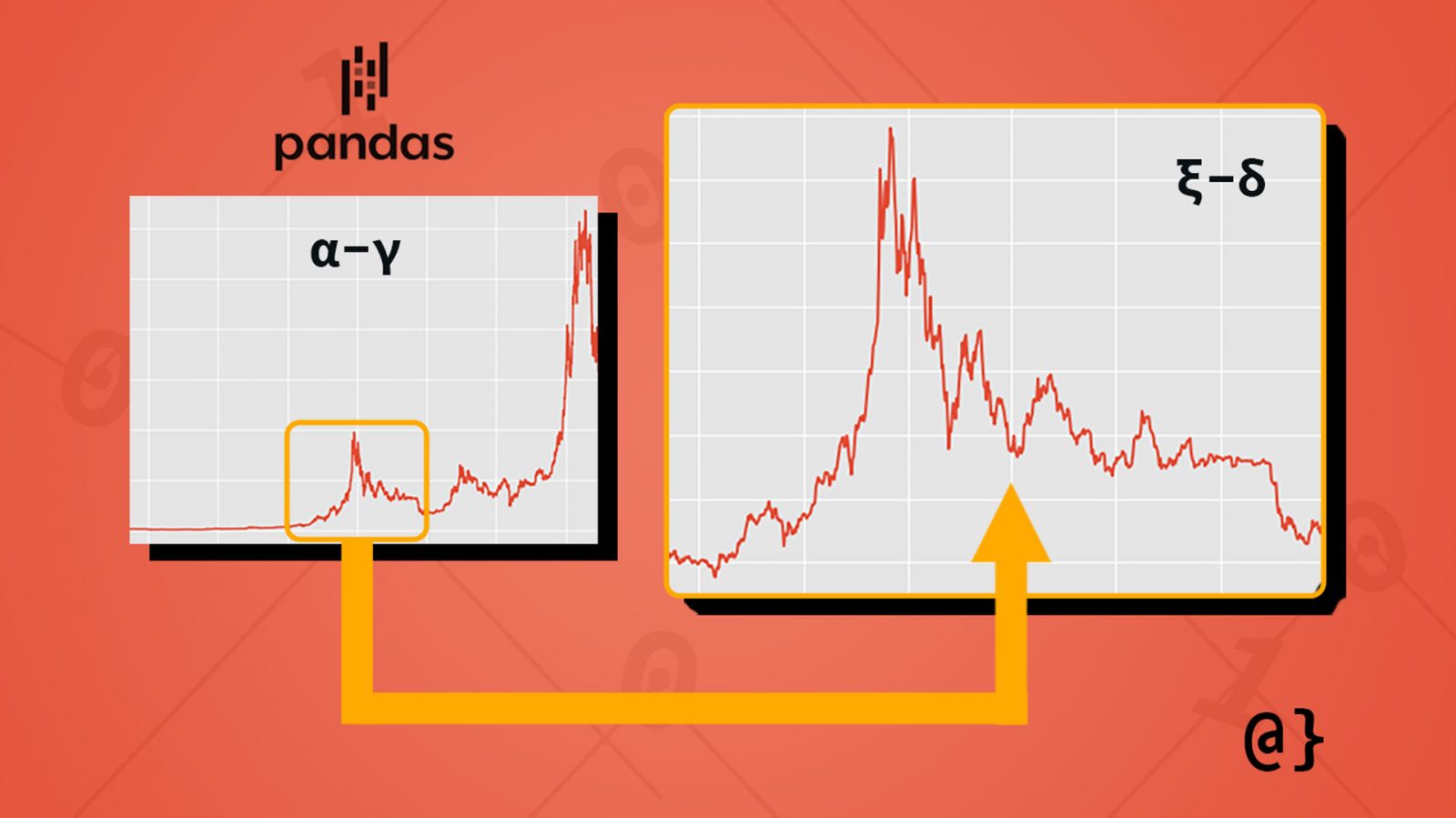
A common issue is that one needs only analyze a subset of dates from a larger Time Series data. In this quick example, we’ll use the .loc method of Pandas DataFrames to select a range of dates from Time Series data.

Selecting a Range of Time Series Dates

Before we select a range of dates from our Time Series in pandas let’s go over some quick assumptions. First and foremost I’m assuming you have loaded data into a DataFrame per standard practices outlined in the official documentation. With that assumption, we also are making the following assumptions:

1. We have data
2. The data is loaded into memory as a DataFrame object
3. The data has an associated sequence of dates

Just so everyone is on the same page, let’s take a look at our data. Below is a Time Series data containing the Adjusted Close price for Bitcoin from the dates 2014-09-17 to 2021-06-26. For the curious, that reflects a relative price increase of 6668.4832%.

# Inspect our data
>>> df

Date
2014-09-17      457.334015
2014-09-18      424.440002
2014-09-19      394.795990
2014-09-20      408.903992
2014-09-21      398.821014
                  ...     
2021-06-22    32505.660156
2021-06-23    33723.027344
2021-06-24    34662.437500
2021-06-25    31637.779297
2021-06-26    30954.576172
Name: Adj Close, Length: 2475, dtype: float64

Check/Set Index Value

The first thing we need to do is to ensure our data is properly indexed by the column containing the date values. This value is often set during instantiation of the DataFrame object by using the index_col argument. It can be set to the index value of the Date column or verbose string name (e.g. “Date”.) We double-check this as follows:

# Check the current index of our data
>>> df.index

DatetimeIndex(['2014-09-17', '2014-09-18', '2014-09-19', '2014-09-20',
               '2014-09-21', '2014-09-22', '2014-09-23', '2014-09-24',
               '2014-09-25', '2014-09-26',
               ...
               '2021-06-17', '2021-06-18', '2021-06-19', '2021-06-20',
               '2021-06-21', '2021-06-22', '2021-06-23', '2021-06-24',
               '2021-06-25', '2021-06-26'],
              dtype='datetime64[ns]', name='Date', length=2475, freq=None)

Optional: Visualize the Data

Just for kicks, let’s visualize this Time Series as a line plot quickly:

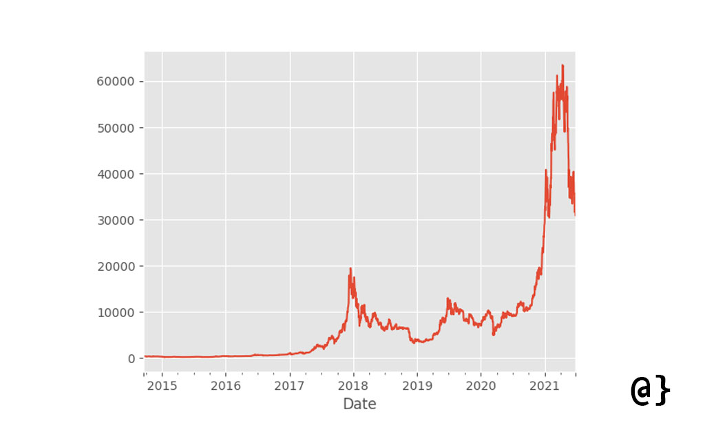
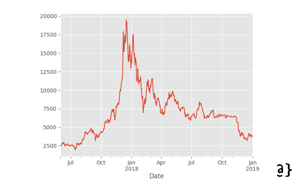
While not strictly necessary for our example here I find plots helpful in assessing which ranges of data one might want to further analyze. In those cases, the period between 2017 and 2019 looks pretty interesting. Let’s isolate that range of Time Series Data in Pandas.

Slice Indexes via .loc Method

There are a number of ways to select ranges from Time Series data in pandas. I find the easiest to be using the .loc operator. It is highly optimized and offers a friendly syntactic use. Let’s slice into our Time Series:

# Select range
>>> data.loc['2017-06-01':'2019-01-01']

Date
2017-06-01    2407.879883
2017-06-02    2488.550049
2017-06-03    2515.350098
2017-06-04    2511.810059
2017-06-05    2686.810059
                 ...     
2018-12-28    3923.918701
2018-12-29    3820.408691
2018-12-30    3865.952637
2018-12-31    3742.700439
2019-01-01    3843.520020
Name: Adj Close, Length: 580, dtype: float64

Our DataFrame Time Series object now contains data restricted to the range of June 1st, 2017 through January 1st, 2019 (the interesting part of the chart above.) Let’s take another look at this chart to confirm visually.

Final Thoughts

This quick example demonstrates how Pandas provides an easy sub-selection of Time Series data by a range of dates. Here we’ve used what Pandas refers to as Partial String Indexing to achieve our desired results. Alternative approaches include using the mask feature. One parting word of advice is that, for those loading Time Series data via CSV files, making use of the parse_dates and index_col arguments will save much heartache.