Predicting stock prices in Python using linear regression is easy. Finding the right combination of features to make those predictions profitable is another story. In this article, we’ll train a regression model using historic pricing data and technical indicators to make predictions on future prices.
We’ll cover how to add technical indicators using the pandas_ta package, how to troubleshoot some common errors, and finally let our trained model loose with a basic trading strategy to assess its predictive power. This article focuses primarily on the implementation of the scikit-learn LinearRegression model and assumes the reader has a basic working knowledge of the Python language.
Highlights
- We’ll get load historic pricing data into a Pandas’
DataFrameand add technical indicators to use as features in our Linear Regression model. - We’ll extract only the data we intend to use from the DataFrame
- We’ll cover some common mistakes in how data is handled prior to training our model and show how some simple “reshaping” can solve a nagging error message.
- We’ll train a simple linear regression model using a 10-day exponential moving average as a predictor for the closing price.
- We’ll analyze the accuracy of our model, plot the results, and consider the magnitude of our errors
- Finally, we’ll run a simulated trading strategy to see what kind of returns we could make by leveraging the predictive power of our model. Spoiler alert: it turned out pretty decent!
Introduction
Linear regression is utilized in business, science, and just about any other field where predictions and forecasting are relevant. It helps identify the relationships between a dependent variable and one or more independent variables. Simple linear regression is defined by using a feature to predict an outcome. That’s what we’ll be doing here.
Stock market forecasting is an attractive application of linear regression. Modern machine learning packages like scikit-learn make implementing these analyses possible in a few lines of code. Sounds like an easy way to make money, right? Well, don’t cash in your 401k just yet.
As easy as these analyses are to implement, selecting features with ample enough predictive power to turn a profit is more of an art than science. In training our model, we’ll take a look at how to easily add common technical indicators to our data to use as features in training our model. Let’s take this in a step-by-step approach starting with getting our historic pricing data.
Note: The information in this article is for informational purposes only and does not constitute financial advice. See our financial disclosure for more information.
Step 1: Get Historic Pricing Data
To get started we need data. This will come in the form of historic pricing data for Tesla Motor’s (TSLA). I’m getting this as a direct .csv download from the finance.yahoo.com website and loading it into memory as a pandas data frame. See this post on getting stock prices with Python for a more detailed walkthrough.
import pandas as pd

# Load local .csv file as DataFrame
df = pd.read_csv('TSLA.csv')

# Inspect the data
print(df)

# List of entries
           Date        Open        High  ...       Close   Adj Close     Volume
0    2020-01-02   84.900002   86.139999  ...   86.052002   86.052002   47660500
1    2020-01-03   88.099998   90.800003  ...   88.601997   88.601997   88892500
2    2020-01-06   88.094002   90.311996  ...   90.307999   90.307999   50665000
3    2020-01-07   92.279999   94.325996  ...   93.811996   93.811996   89410500
4    2020-01-08   94.739998   99.697998  ...   98.428001   98.428001  155721500
..          ...         ...         ...  ...         ...         ...        ...
248  2020-12-24  642.989990  666.090027  ...  661.770020  661.770020   22865600
249  2020-12-28  674.510010  681.400024  ...  663.690002  663.690002   32278600
250  2020-12-29  661.000000  669.900024  ...  665.989990  665.989990   22910800
251  2020-12-30  672.000000  696.599976  ...  694.780029  694.780029   42846000
252  2020-12-31  699.989990  718.719971  ...  705.669983  705.669983   49649900

[253 rows x 7 columns]

# Show some summary statistics
print(df.describe())

             Open        High         Low       Close   Adj Close        Volume
count  253.000000  253.000000  253.000000  253.000000  253.000000  2.530000e+02
mean   289.108428  297.288412  280.697937  289.997067  289.997067  7.530795e+07
std    167.665389  171.702889  163.350196  168.995613  168.995613  4.013706e+07
min     74.940002   80.972000   70.101997   72.244003   72.244003  1.735770e+07
25%    148.367996  154.990005  143.222000  149.792007  149.792007  4.713450e+07
50%    244.296005  245.600006  237.119995  241.731995  241.731995  7.025550e+07
75%    421.390015  430.500000  410.579987  421.200012  421.200012  9.454550e+07
max    699.989990  718.719971  691.119995  705.669983  705.669983  3.046940e+08
Note: This data is available for download via Github.
Step 2: Prepare the data
Before we start developing our regression model we are going to trim our data some. The ‘Date’ column will be converted to a DatetimeIndex and the ‘Adj Close’ will be the only numerical values we keep. Everything else is getting dropped.
# Reindex data using a DatetimeIndex
df.set_index(pd.DatetimeIndex(df['Date']), inplace=True)

# Keep only the 'Adj Close' Value
df = df[['Adj Close']]

# Re-inspect data
print(df)

             Adj Close
Date
2020-01-02   86.052002
2020-01-03   88.601997
2020-01-06   90.307999
2020-01-07   93.811996
2020-01-08   98.428001
...                ...
2020-12-24  661.770020
2020-12-28  663.690002
2020-12-29  665.989990
2020-12-30  694.780029
2020-12-31  705.669983

[253 rows x 1 columns]

# Print Info
print(df.info())

<class 'pandas.core.frame.DataFrame'>
DatetimeIndex: 253 entries, 2020-01-02 to 2020-12-31
Data columns (total 1 columns):
 #   Column     Non-Null Count  Dtype
---  ------     --------------  -----
 0   Adj Close  253 non-null    float64
dtypes: float64(1)
memory usage: 4.0 KB
What we see here is our ‘Date’ column having been converted to a DatetimeIndex with 253 entries and the ‘Adj Close’ column being the only retained value of type float64 (np.float64.) Let’s plot our data to get a visual picture of what we’ll be working with from here on out.
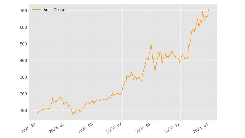
We can see a significant upward trend here reflecting a 12-month price increase from 86.052002 to 705.669983. That’s a relative increase of ~720%. Let’s see if we can’t develop a linear regression model that might help predict upward trends like this!
Aside: Linear Regression Assumptions & Autocorrelation
Before we proceed we need to discuss a technical limitation of linear regression. Linear regression requires a series of assumptions to be made to be effective. One can certainly apply a linear model without validating these assumptions but useful insights are not likely to be had.
One of these assumptions is that variables in the data are independent. Namely, this dictates that the residuals (difference between the predicted value and observed value) for any single variable aren’t related.
For Time Series data this is often a problem since our observed values are longitudinal in nature—meaning they are observed values for the same thing, recorded in sequence. This produces a characteristic called autocorrelation which describes how a variable is somehow related to itself (self-related.) (Chatterjee, 2012)
Autocorrelation analysis is useful in identifying trends like seasonality or weather patterns. When it comes to extrapolating values for price prediction, however, it is problematic. The takeaway here is that our date values aren’t suitable as our independent variable and we need to come up with something else and use the adjusted close value as the independent variable. Fortunately, there are some great options here.
Step 3: Adding Technical Indicators
Technical indicators are calculated values describing movements in historic pricing data for securities like stocks, bonds, and ETFs. Investors use these metrics to predict the movements of stocks to best determine when to buy, sell, or hold.
Commonly used technical indicators include moving averages (SMA, EMA, MACD), the Relative Strength Index (RSI), Bollinger Bands (BBANDS), and several others. There is certainly no shortage of popular technical indicators out there to choose from. To add our technical indicators we’ll be using the pandas_ta library. To get started, let’s add an exponential moving average (EMA) to our data:
import pandas_ta

# Add EMA to dataframe by appending
# Note: pandas_ta integrates seamlessly into
# our existing dataframe
df.ta.ema(close='adj_close', length=10, append=True)

# Inspect Data once again
             adj_close      EMA_10
date
2020-01-02   86.052002         NaN
2020-01-03   88.601997         NaN
2020-01-06   90.307999         NaN
2020-01-07   93.811996         NaN
2020-01-08   98.428001         NaN
...                ...         ...
2020-12-24  661.770020  643.572394
2020-12-28  663.690002  647.230141
2020-12-29  665.989990  650.641022
2020-12-30  694.780029  658.666296
2020-12-31  705.669983  667.212421

[253 rows x 2 columns]

<class 'pandas.core.frame.DataFrame'>
DatetimeIndex: 253 entries, 2020-01-02 to 2020-12-31
Data columns (total 2 columns):
 #   Column     Non-Null Count  Dtype
---  ------     --------------  -----
 0   adj_close  253 non-null    float64
 1   EMA_10     244 non-null    float64
dtypes: float64(2)
As evident from the printouts above, we now have a new column in our data titled “EMA_10.” This is our newly-calculated value representing the exponential moving average calculated over a 10-day period.
Note: The pandas_ta library will alter the column names. Here we see the “Adj Close” column renamed to “adj_close.” This is expected behavior but can cause issues if one isn’t aware of this functionality.
This is great news but also comes with a caveat: the first 9 entries in our data will have a NaN value since there weren’t proceeding values from which the EMA could be calculated. Let’s take a closer look at that:
# Print the first 10 entries of our data
print(df.head(10))

             adj_close     EMA_10
date
2020-01-02   86.052002        NaN
2020-01-03   88.601997        NaN
2020-01-06   90.307999        NaN
2020-01-07   93.811996        NaN
2020-01-08   98.428001        NaN
2020-01-09   96.267998        NaN
2020-01-10   95.629997        NaN
2020-01-13  104.972000        NaN
2020-01-14  107.584000        NaN
2020-01-15  103.699997  96.535599
We need to deal with this issue before moving on. There are several approaches we could take to replace the NaN values in our data. These include replacing with zeros, the mean for the series, backfilling from the next available, etc. All these approaches seek to replace NaN values with some pseudo values.
Given our goal of predicting real-world pricing that’s not an attractive option. Instead, we’re going to just drop all the rows where we have NaN values and use a slightly smaller dataset by taking the following approach:
# Drop the first n-rows
df = df.iloc[10:]

# View our newly-formed dataset
print(df.head(10))

             adj_close      EMA_10
date
2020-01-16  102.697998   97.656035
2020-01-17  102.099998   98.464028
2020-01-21  109.440002  100.459660
2020-01-22  113.912003  102.905540
2020-01-23  114.440002  105.002715
2020-01-24  112.963997  106.450221
2020-01-27  111.603996  107.387271
2020-01-28  113.379997  108.476858
2020-01-29  116.197998  109.880701
2020-01-30  128.162003  113.204574
Now we’re ready to start developing our regression model to see how effective the EMA is at predicting the price of the stock. First, let’s take a quick look at a plot of our data now to get an idea of how the EMA value tracks with the adjusted closing price.
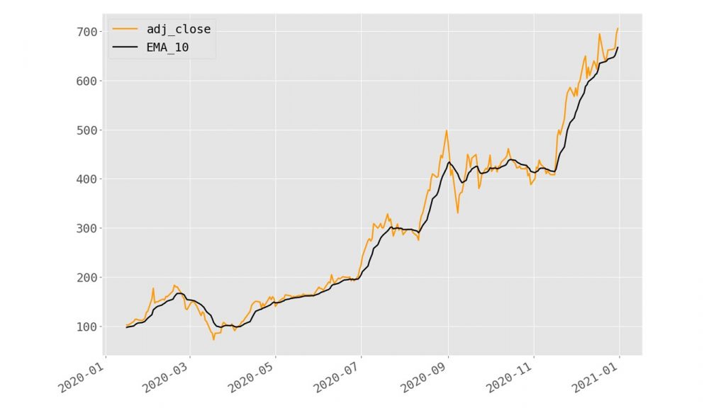
We can see here the EMA tracks nicely and that we’ve only lost a littttttle bit of our data at the leading edge. Nothing to worry about—our linear model will still have ample data to train on!
Step 4: Test-Train Split
Machine learning models require at minimum two sets of data to be effective: the training data and the testing data. Given that new data can be hard to come by, a common approach to generate these subsets of data is to split a single dataset into multiple sets (Xu, 2018).
Using eighty percent of data for training and the remaining twenty percent for testing is common. This 80/20 split is the most common approach but more formulaic approaches can be used as well (Guyon, 1997).
The 80/20 split is where we’ll be starting out. Rather than mucking about trying to split our DataFrame object manually we’ll just the scikit-learn test_train_split function to handle the heavy lifting:
# Split data into testing and training sets
X_train, X_test, y_train, y_test = train_test_split(df[['adj_close']], df[['EMA_10']], test_size=.2)

# Test set
print(X_test.describe())

          adj_close
count     49.000000
mean     272.418612
std      140.741107
min       86.040001
25%      155.759995
50%      205.009995
75%      408.089996
max      639.830017

# Training set
print(X_train.describe())

          adj_close
count    194.000000
mean     291.897732
std      166.033359
min       72.244003
25%      155.819996
50%      232.828995
75%      421.770004
max      705.669983
We can see that our data has been split into separate DataFrame objects with the nearest whole-number value of rows reflective of our 80/20 split (49 test samples, 192 training samples.) Note the test size 0.20 (20%) was specified as an argument to the train_test_split function.
Note: The X_train, X_test, y_train, and y_test data are Pandas DataFrame objects in memory. This results from the use of double-bracketed access notation df[['adj_close']] as opposed to single-bracket notation df['adj_close']. The single-bracketed notation would return a Series object and would require reshaping before we could proceed to fit our model. See this post for more details.
Step 5: Training the Model
We have our data and now we want to see how well it can be fit to a linear model. Scikit-learn’s LinearRegression class makes this simple enough—requiring only 2 lines of code (not including imports):
from sklearn.linear_model import LinearRegression

# Create Regression Model
model = LinearRegression()

# Train the model
model.fit(X_train, y_train)

# Use model to make predictions
y_pred = model.predict(X_test)
That’s it—our linear model has now been trained on 194 training samples, and we’ve generated predicted values (y_pred). Now we can assess how well our model fits our data by examining our model coefficients and some statistics like the mean absolute error (MAE) and coefficient of determination (r2).
Step 6: Validating the Fit
The linear model generates coefficients for each feature during training and returns these values as an array. In our case, we have one feature that will be reflected by a single value. We can access this using the model.regr_ attribute.
In addition, we can use the predicted values from our trained model to calculate the mean squared error and the coefficient of determination using other functions from the sklearn.metrics module. Let’s see a medley of metrics useful in evaluating our model’s utility.
from sklearn.metrics import mean_squared_error, r2_score, mean_absolute_error

# Printout relevant metrics
print("Model Coefficients:", model.coef_)
print("Mean Absolute Error:", mean_absolute_error(y_test, y_pred))
print("Coefficient of Determination:", r2_score(y_test, y_pred))

# Results
Model Coefficients: [[0.94540376]]
Mean Absolute Error: 12.554147460577513
Coefficient of Determination: 0.9875188616393644
The MAE is the arithmetic mean of the absolute errors of our model, calculated by summing the absolute difference between observed values of X and Y and dividing by the total number of observations.
The MAE can be described as the sum of the absolute error for all observed values divided by the total number of observations. Check out this article by Shravankumar Hiregoudar for a deeper look into using the MAE, as well as other metrics, for evaluating regression models.
For now, let’s just recognize that a lower MAE value is better, and the closer our coefficient of the correlation value is to 1.0 the better. The metrics here suggest that our model fits our data well, though the MAE is slightly high.
Let’s consider a chart of our observed values compared to the predicted values to see how this is represented visually:
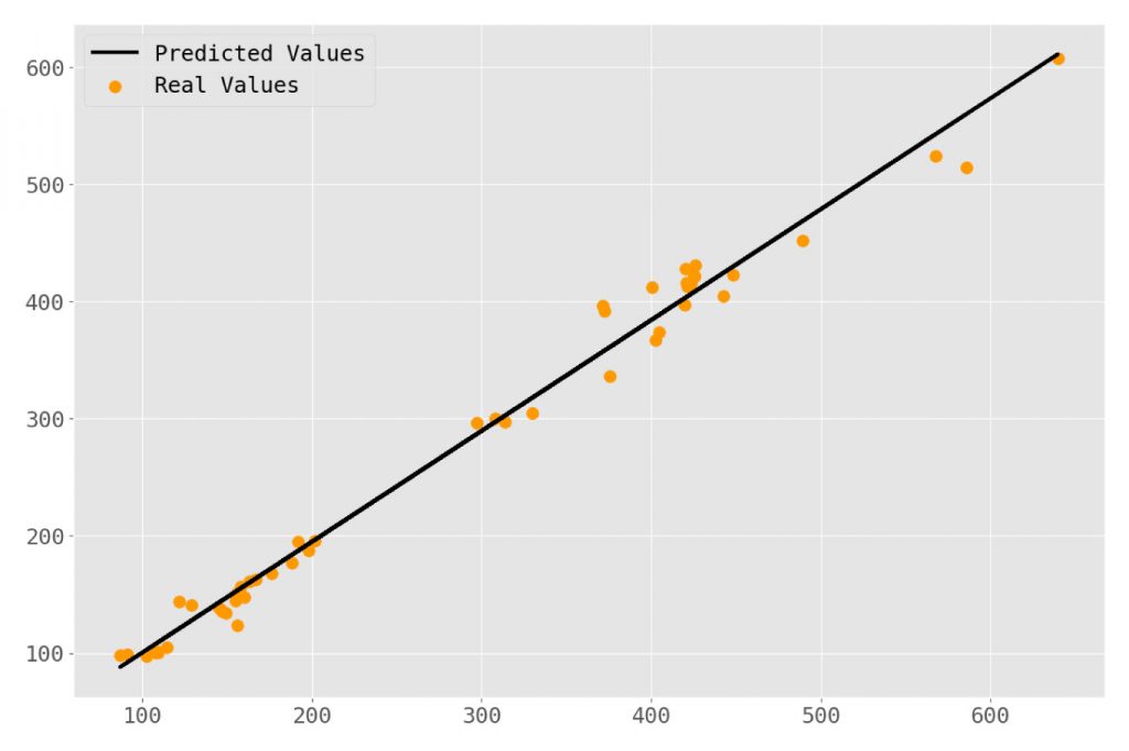
This looks like a pretty good fit! Given our relatively high r2 value that’s no surprise. Just for kicks, let’s add some lines to represent the residuals for each predicted value.
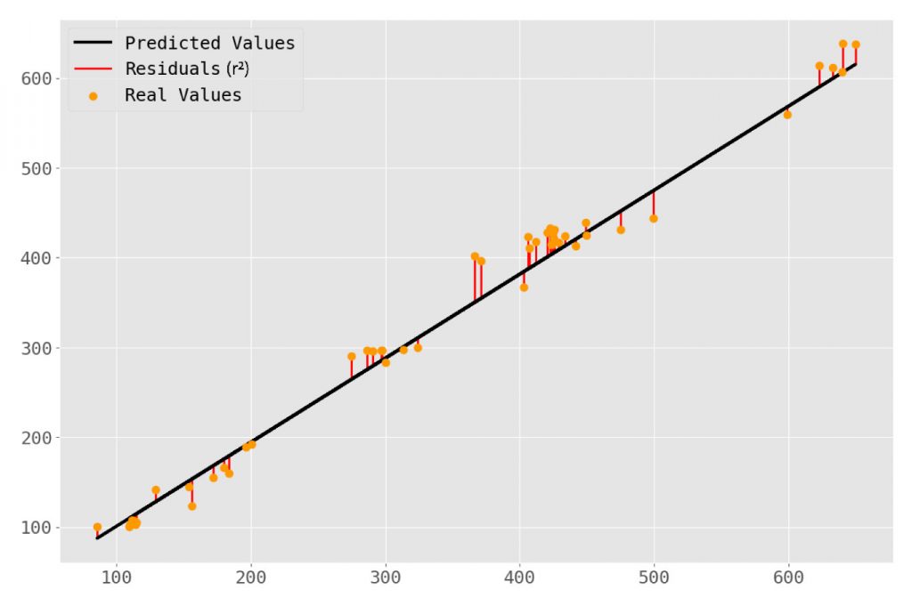
This doesn’t tell us anything new but helps to conceptualize what the coefficient of correlation is actually representing—an aggregate statistic for how far off our predicted values are from the actual values. So now we have this linear model—but what is it telling us?
Step 7: Interpretation
At this point, we’ve trained a model on historical pricing data using the Adjusted Closing value and the Exponential Moving Average for a 10-day trading period. Our goal was to develop a model that can use the EMA of any given day (dependent on pricing from the previous 9 days) and accurately predict that day’s closing price. Let’s run a simulation of a very simple trading strategy to assess how well we might have done using this.
Strategy: If our model predicts a higher closing value than the opening value we make a trade for a single share on that day—buying at market open and selling just before market close.
Below is a summary of each trading day during our test data period:
Results
In the 49 possible trade days, our strategy elected to make 4 total trades. This strategy makes two bold assumptions:
- We were able to purchase a share at the exact price open price recorded;
- We were able to sell that share just before closing at the exact price recorded.
Applying this strategy—and these assumptions—our model generated $151.77. If our starting capital was $1,000 this strategy would have resulted in a ~15.18% increase of total capital.
Shortcomings
Before you open your TD Ameritrade account and start transferring your 401K let’s consider these results—there are quite a few problems with them after all.
- We’re applying this model to data very close to the training data;
- We aren’t accounting for relevant broker fees for buy/sells
- We aren’t accounting for taxes—as much as your “ordinary income” as the IRS would say.
Review
Using linear regression to predict stock prices is a simple task in Python when one leverages the power of machine learning libraries like scikit-learn. The convenience of the pandas_ta library also cannot be overstated—allowing one to add any of the dozens of technical indicators in single lines of code.
In this article we have seen how to load in data, test-train split the data, add indicators, train a linear model, and finally apply that model to predict future stock prices—with some degree of success!
The use of the exponential moving average (EMA) was chosen somewhat arbitrarily. There are many other technical indicators that are common among algorithmic trading and traditional trading strategies:
- Relative Strenght Index
- Mean Average Convergence-Divergence (MACD)
- Aspects of Bollinger Bands
- Average Daily Range or Average True Range
- so many more …
These indicators can be used instead of the EMA, alongside it in multiple regression models, or creatively combined with feature engineering. The only limitation to how one chooses to leverage these indicators in developing linear models is imagination alone!
References
- Chatterjee. Regression Analysis by Example, 5th Edition. 5th ed., Wiley, 2012.
- Guyon, Isabelle. A Scaling Law for the Validation-Set Training-Set Size Ratio. In AT & T Bell Laboratories. (1997) doi:10.1.1.33.1337
- Xu, Yun, and Royston Goodacre. “On Splitting Training and Validation Set: A Comparative Study of Cross-Validation, Bootstrap and Systematic Sampling for Estimating the Generalization Performance of Supervised Learning.” Journal of analysis and testing vol. 2,3 (2018): 249-262. doi:10.1007/s41664-018-0068-2


