3 Easy Ways to Get Financial Data in Python for Stock Analysis

Python is often used for algorithmic trading, backtesting, and stock market analysis. In fact, it seems almost the canonical use-case for many tutorials I’ve seen over the years. Getting financial data in Python is the prerequisite skill for any such analysis.

In this article, you’ll learn how to easily get, read, and interpret financial data using Python. We’ll be using the Pandas library, the yfinance library, and a handful of useful helper methods. Readers should be familiar with basic Python syntax but needn’t have obtained a level of skill mistakable as guru.

Highlights

• Understanding structured vs. unstructured financial data
• What is OHLC data
• Popular Python financial libraries
• Getting data from various sources via Python including Yahoo Finance, Quandl, and Alpha Vantage
• Deprecated APIs such as Google Finance

Financial Data 101

Financial data comes in many forms. The canonical format is tabular data (think spreadsheets) which can be formatted as rows and columns. This type of data is available from many sources such as finance.yahoo.com, Quandl, Alpha Vantage, and many brokerages.

Financial data can be bought, manually scraped from the web, or obtained from public APIs. Generally, financial data comes in one of 2 primary types:

• Structured Data: Closing prices, financials, market performance, etc.
• Unstructured Data: News articles, Social Media, Sentiment Analysis, etc.

Additionally, financial data can be further categorized as either Historical or Real-Time. In most cases, Real-Time data isn’t available from public APIs and must be purchased. We’ll be using mostly structured historical data for our examples here. These financial data are generally provided in a format that includes the following information:

• Date
• Open Price
• High Price
• Low Price
• Closing Price
• Volume

These data—often referred to as OHLC Chart Data—can be interpreted as Time Series data and are perfect for performing technical analysis. We’ll dive into this format in just a moment but, for now, just realize this is a standard format for historical pricing data within financial markets.

Pandas

Pandas is a powerful data science library that stores tabular data into memory in a very efficient manner. It makes the opening, processing, and subsequent saving of data fast and effective. It comes with a range of helper methods, data classes, and in the case of financial data—web APIs!

This article will glaze over much of the intricacies of the Pandas library—just know that it is complex! We will be mostly using the data_reader function, the DataFrame class, and miscellaneous statistic-generating functions like head(), info(), summary() and etc.

Required Libraries

Now that we know what to expect from our data, let’s consider how to get some financial data using Python! Before we get started, make sure the following packages are installed as they will be relevant for each data source. We’ll cover specific packages as we move along.

# Install the pandas library
pip install pandas

# Install the pandas-datareader library
# Note: Will also install pandas if not already installed.
pip install pandas-datareader

Yahoo Finance

Pros:

• Free
• Huge amount of data
• Well-supported Python libraries
• Integrated with many backtesting libraries

Cons:

• No official API is available
• Basic data only
• Can get IP rate-limited or banned

Yahoo Finance provides historical data for a massive number of securities. You’ll find data for securities, currencies, and even cryptocurrencies like Bitcoin ($BTC-USD). We can use the pandas-datareader library as well as the yfinance library to get financial data from Yahoo Finance. Let’s consider both approaches:

Note: I would suggest using a proxy when accessing yahoo financial data. Both the yfinance library and pandas-datareader libraries accommodate this.

Using Pandas-Datareader

import pandas_datareader as pdr

# Request data via Yahoo public API
data = pdr.get_data_yahoo('NVDA')

# Display Info
print(data.info())

<class 'pandas.core.frame.DataFrame'>
DatetimeIndex: 1258 entries, 2016-08-08 to 2021-08-05
Data columns (total 6 columns):
 #   Column     Non-Null Count  Dtype  
---  ------     --------------  -----  
 0   High       1258 non-null   float64
 1   Low        1258 non-null   float64
 2   Open       1258 non-null   float64
 3   Close      1258 non-null   float64
 4   Volume     1258 non-null   float64
 5   Adj Close  1258 non-null   float64
dtypes: float64(6)
memory usage: 68.8 KB

Here we see a 5-year historical period of OHLC data for $NVDA (NVidia Corporation) provided as a pandas’ DataFrame object with 1258 rows of data. Excluding imports and summaries—that took a single line of code.

Using yfinance

For this approach, we need to install the yfinance library as pip install yfinance. This library provides ample tools for working with financial data requests to the Yahoo Finance website. Keep in mind, however, this is not an official API and is subject to rate limiting, periodic breakage, and general quirkiness. Nonetheless, its the defacto Python library for OHLC data and can be used as follows:

import yfinance as yf

# Request historical data for past 5 years
data = yf.Ticker("NVDA").history(period='5y')

# Show info
print(data.info())

<class 'pandas.core.frame.DataFrame'>
DatetimeIndex: 1258 entries, 2016-08-08 to 2021-08-05
Data columns (total 7 columns):
 #   Column        Non-Null Count  Dtype  
---  ------        --------------  -----  
 0   Open          1258 non-null   float64
 1   High          1258 non-null   float64
 2   Low           1258 non-null   float64
 3   Close         1258 non-null   float64
 4   Volume        1258 non-null   int64  
 5   Dividends     1258 non-null   float64
 6   Stock Splits  1258 non-null   float64
dtypes: float64(6), int64(1)
memory usage: 78.6 KB

Here we see the same 5-year historical data for $NVDA returned as the familiar pandas’ DataFrame object. We’ve used a little more complex syntax but achieved the same basic result. The yfinance library’s Ticker class doesn’t actually retrieve data. The history method helps us with that and takes a number of optional parameters.

By default, yfinance returns a previous months’ data as a daily time series. Note this method adds two additional columns: Dividends and Stock Splits; and also omits the adjusted close column. The Adjusted Close data takes into account such actions a dividends payouts and stock splits. The inclusion here assumes we’re comfortable calculating our own adjusted close.

Quandl

Pros:

• Free to use (rate limited)
• Datasets can be downloaded
• Official Python Library
• Good API documentation

Cons:

• Limited OHLC data
• No real-time or delayed data for stocks
• A limited number of free datasets
• Free API access for non-rate limited use (or freer access at least)

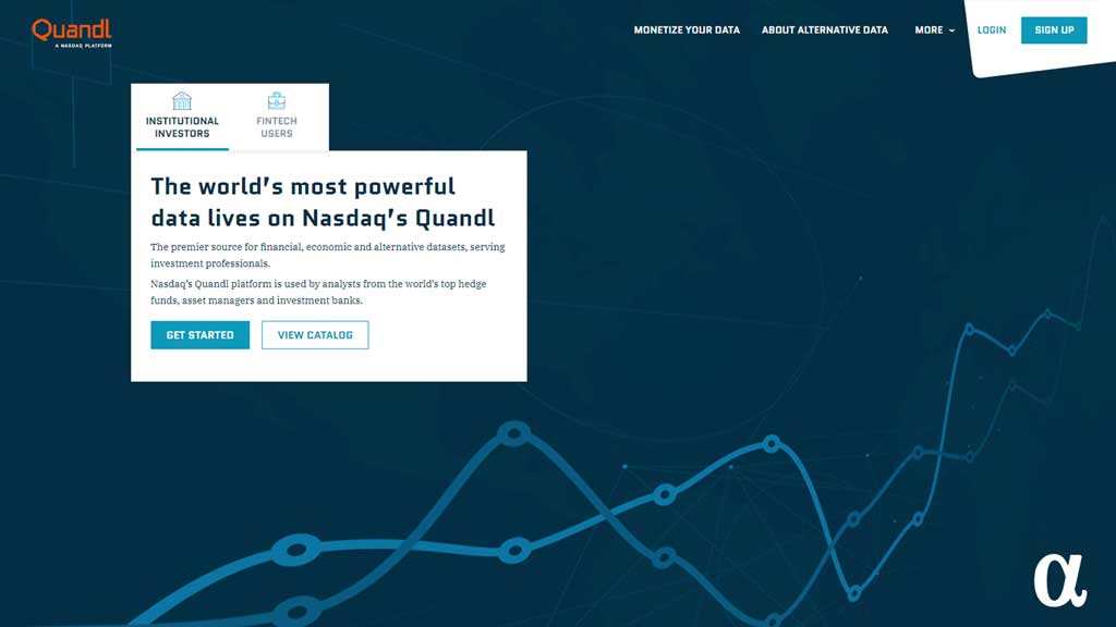
Quandl is one of the largest data providers in the world. Their self-confessed mission is the “inspire customers to make new discoveries and incorporate them into trading strategies.” They’ve been around since 2013 and offer millions of free datasets. Yes, millions.

In 2018 they were acquired by NASDAQ and have continued to remain an authority on financial data ranging from equities and futures to options, currencies, and other non-financial market data such as housing, energy, and agriculture.

Quandl offers official APIs to access any public dataset for free. Here we’ll see how to get OHLC data via the official Quandl python library and also via the pandas-datareader. One important note is that the free Quandl OHLC data only goes up to 2018 at the time of this article’s writing. If you need more recent data and don’t want to pay this source isn’t for you.

Quandl Python Library

To get started with Quadl’s official API we need to install the python library as such: pip install quandl. This will install the official quandl python library and let us make up to 50 daily API requests without registering an account. Let’s get our financial data:

import quandl

# Get data via Quandl API
data = quandl.get('WIKI/NVDA')

# Summarize
print(data.info())

<class 'pandas.core.frame.DataFrame'>
DatetimeIndex: 4825 entries, 1999-01-22 to 2018-03-27
Data columns (total 12 columns):
 #   Column       Non-Null Count  Dtype  
---  ------       --------------  -----  
 0   Open         4825 non-null   float64
 1   High         4825 non-null   float64
 2   Low          4825 non-null   float64
 3   Close        4825 non-null   float64
 4   Volume       4825 non-null   float64
 5   Ex-Dividend  4825 non-null   float64
 6   Split Ratio  4825 non-null   float64
 7   Adj. Open    4825 non-null   float64
 8   Adj. High    4825 non-null   float64
 9   Adj. Low     4825 non-null   float64
 10  Adj. Close   4825 non-null   float64
 11  Adj. Volume  4825 non-null   float64
dtypes: float64(12)
memory usage: 490.0 KB

Our data is similar to before; it’s still a pandas’ DataFrame object, it still contains rows and columns, but we’ve got a lot more of it. By default, the quandl API returns all available data for the requested asset. Date ranges can be specified using a start_date="YYYY-MM-DD" and end_date="YYYY-MM-DD" pair of keyword arguments to the get method.

Note that our ticker syntax has changed a bit from the yfinance example. Instead of requesting “NVDA” we’re now requesting “WIKI/NVDA.” This syntax instructs the Quandl API to query the WIKI dataset for an entry labeled NVDA. Read the documentation for more on that.

pandas-datareader

As with the Yahoo Finance data, the pandas-datareader library also accommodates requests to the Quandl API. However, this approach requires that one have an API key to provide as an argument. API keys are free, don’t require any payment methods to be stored, and can be obtained via the Quandl signup page.

Note: you will have to confirm your email address before the key becomes active. With our API key in hand, we can get data via the pandas-datareader library as such:

# Necessary imports
import pandas_datareader as pdr

# Request Data
data = pdr.get_data_quandl("NVDA", api_key="YoUrApIkEyGoEsHeRe")

# Summarize
print(data.info())

<class 'pandas.core.frame.DataFrame'>
DatetimeIndex: 411 entries, 2018-03-27 to 2016-08-08
Data columns (total 12 columns):
 #   Column      Non-Null Count  Dtype  
---  ------      --------------  -----  
 0   Open        411 non-null    float64
 1   High        411 non-null    float64
 2   Low         411 non-null    float64
 3   Close       411 non-null    float64
 4   Volume      411 non-null    float64
 5   ExDividend  411 non-null    float64
 6   SplitRatio  411 non-null    float64
 7   AdjOpen     411 non-null    float64
 8   AdjHigh     411 non-null    float64
 9   AdjLow      411 non-null    float64
 10  AdjClose    411 non-null    float64
 11  AdjVolume   411 non-null    float64
dtypes: float64(12)
memory usage: 41.7 KB

Here we see another familiar image: historic OHLC data provided as a pandas’ DataFrame class object. The QuandlReader class in pandas-datareader will default to the WIKI dataset if only a ticker is provided. This makes for convenient OHLV requests but may cause some confusion when trying to retrieve data from other datasets. Just stick to the Quandl-recommended syntax of DATASET/QUERY for those.

Alpha Vantage

Pros:

• Free to use
• Large Amounts of Datasets
• Offers Technical Indicators
• Good API documentation
• Intraday Data

Cons:

• Rate limiting of API access
• Real-Time Data is delayed

Alpha Vantage supplies a myriad of free data via API access. These data are free but not public meaning you need an API key. Such keys can be obtained by registering an account with Alpha Vantage. Entering your name, email, and status (educator, student, investor, etc.) will earn you an API key in a matter of seconds—you don’t even have to confirm your email! Let’s take a look at getting data from this API.

Unofficial Python alpha_vantage API

There is not official Python library for the Alpha Vantage API and their official documentation only details common HTTP requests via the requests module. This approach is 100% valid and will provide the OHLC data without issue. Syntactically, it’s a bit more cumbersome.

In pursuit of some sugar for our syntactic sweet tooth, we’ll use the well-developed alpha_vantage library. This is an unofficial API but, at least in my experience, the defacto Python Alpha Vantage API library. Let’s see how this library can retrieve our OHLC data:

from alpha_vantage.timeseries import TimeSeries

# Create an API object
ts = TimeSeries(key='UNO4CZQHSBZSN71N')
print(type(ts))

# Get daily OHLC data for NVDA
data, meta_data = ts.get_daily(symbol="NVDA")
print(data)

{
    '2021-08-05': {
        '1. open': '205.0000',
        '2. high': '207.3300',
        '3. low': '203.4200',
        '4. close': '206.3700',
        '5. volume': '21143537'
    },
    '2021-08-04': {
        '1. open': '199.9000',
        '2. high': '203.1800',
        '3. low': '198.2800',
        '4. close': '202.7400',
        '5. volume': '23130940'
    },

    ...

    '2021-03-16': {
        '1. open': '534.2600',
        '2. high': '540.5000',
        '3. low': '524.6700',
        '4. close': '531.6500',
        '5. volume': '6803240'
    }
}

We can see here the last several month’s worths of OHLC data from the Alpha Vantage database. However, we’ve got our first curveball: our data is returned as a dictionary object rather than the pandas DataFrame class object we’ve come to know and love. To get back to the basics, we need only supply the following argument to the TimeSeries object instantiation: output_format='pandas'. With that, our data looks like this:

            1. open  2. high    3. low  4. close   5. volume
date                                                        
2021-08-05   205.00   207.33  203.4200    206.37  21143537.0
2021-08-04   199.90   203.18  198.2800    202.74  23130940.0
2021-08-03   197.40   202.22  192.2000    198.15  30181074.0
2021-08-02   197.00   199.61  193.6100    197.50  21744397.0
2021-07-30   194.18   196.30  192.6300    194.99  18349746.0
...             ...      ...       ...       ...         ...
2021-03-22   516.51   535.78  516.2700    527.45   7445077.0
2021-03-19   510.00   516.86  504.5000    513.83   7480174.0
2021-03-18   525.46   527.36  508.6817    508.90   7354702.0
2021-03-17   521.59   538.13  519.5800    533.65   6096605.0
2021-03-16   534.26   540.50  524.6700    531.65   6803240.0

[100 rows x 5 columns]

Ahh, that’s much better. Now we can see that we have a 5-column DataFrame with 100 rows. To get more than the previous 100 periods’ worth of data, you can use the outputsize='full' argument in the ts.get_daily() method. This will return all available data.

pandas-datareader Alpha Vantage API

Again, the pandas-datareader library offers easy access to OHLC data via Alpha Vantage integration. The following code will retrieve historical data for $NVDA once again:

import pandas_datareader as pdr

# Get Alpha Vantage Data
data = pdr.get_data_alphavantage("NVDA", api_key='EnTeRYoUrApIKeYhErE')

# Summarize
print(data.info())

Index: 5027 entries, 2001-08-13 to 2021-08-05
Data columns (total 5 columns):
 #   Column  Non-Null Count  Dtype  
---  ------  --------------  -----  
 0   open    5027 non-null   float64
 1   high    5027 non-null   float64
 2   low     5027 non-null   float64
 3   close   5027 non-null   float64
 4   volume  5027 non-null   int64  
dtypes: float64(4), int64(1)
memory usage: 235.6+ KB

Here we see historic OHLC data for $NVDA all the way back to 2001. This is much more data than the default method of other approaches so be prepared to filter as necessary via the start or end functions. Note: the pandas-datareader get_alphavantage method uses the TIME_SERIES_DAILY argument by default. Consult the Alpha Vantage API documentation for more information on alternatives.

Google

Pros:

• Integrates with Google Sheets

Cons:

• Not available via API
• No Python library
• Officially shut down in 2012

As of October 2012 Google no longer offers a financial API service. This news came as a shock to many but was ultimately reflective of many policy changes to public APIs. Google also does not provide financial data via metered APIs, as evidenced by a search on their APIs explorer. The Google Finance API is still available however but only as an Excel-style formula in Google Sheets:

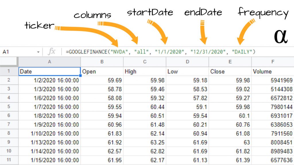
This isn’t a Python-centric way of getting financial data and is included here only because of historical relevancy. I suppose one could hack together an HTTP request method in Python for this—but that’s beyond the scope of this article. Check out the official Google Documentation for more information and syntax related to the GOOGLEFINANCE function in sheets.

Using the Data

Getting historical stock prices in Python is all well and good but what is one to do with such data? There are tones of approaches for analyzing OHLC data—allowing one to distill many numbers of useful insights based on expected outcomes and use-case. Below are some projects that can get you started:

• Predicting Stock Prices in Python with Linear Regression
• Calculating the Moving Average Convergence Divergence (MACD) in Python
• Using the Stochastic Oscillator for Algorithmic Trading in Python
• Visualizing Autocorrelation in Time Series Data with Python
• Correlation Analysis with Heatmaps & Matrices in Python

These are only a few common applications of OHLC financial data in Python. These tutorials details how stock data can be used to identify patterns, correlations, and even predict future prices—all in the comfort of Python! Ultimately the only limitation to use of these data is the analyst’s imagination!

Review

We’ve seen here that getting financial data in Python can be approached in many ways. Whether via official APIs, well-supported third-party libraries, or even hacked-together approaches there seems no shortage of OHLC data to be had. These examples showcase why Python has emerged as the defacto programming language for data science—financial data included.

The yahoo finance API, particularly via the yfinance library, is deeply integrated within many backtesting frameworks. As such, it’s been my experience that this library is the defacto source for daily OHLC historic data. It’s not suited for intraday analysis or real-time but proves invaluable for basic analysis.

The data sources here are not meant to be an exhaustive list and are only reflective of common sources available with easy access (minus Google of course.) Some sources provide downloads such that local data can be retained for more efficient loading when entire universes of Stocks are being analyzed. The web-based access APIs discussed here are great for casual testing and on-the-go development.