Pandas is a powerful data science library with heavy optimizations done. The DataFrame object is an efficient data structure whereby data is organized in a 2-dimensional manner with powerful built-in tools for manipulating that data.
The Pandas DataFrame object is useful for displaying, analyzing, and manipulating tabulated data such as spreadsheets. However, sometimes viewing the data can be burdensome in a terminal. In this quick tutorial, we’ll convert a Pandas DataFrame object into a local CSV file for convenient viewing in other programs as well as data storage.
TL; DR
Convert a DataFrame to CSV by using the following code:
# Note: 'df' is an existing DataFrame object
df.to_csv("your-filename.csv")
Load a CSV file as a DataFrame object using the following code:
import pandas as pd

# load local csv; optinally specify column to use as index
df = pd.read_csv("your-filename.csv", index_col='Your Index')
For those looking for a deeper understanding of the processes of saving/converting a DataFrame to CSV or loading a CSV file as a DataFrame, let’s take a look at what this tutorial will cover.
Highlights
By the end of this tutorial, we will have covered the following:
- Fetching remote pricing data via the
yfinancelibrary as a DataFrame object. - Saving the
DataFrameto a local CSV file. - Loading the local CSV file as a
DataFrame. - Reindexing the
DataFrameby the original column rather than row number.
Project Setup
To demonstrate saving a Pandas DataFrame to a .csv file we need to load test data. Below is the code for downloading some historical pricing data for Ether from Yahoo finance via the yfinance python library (pip install yfinance):
import yfinance as yf

# download 1-year daily pricing data for Ether, limit columns
data = yf.Ticker("ETH-USD").history(period='1y', interval='1d')[['Open', 'High', 'Low', 'Close', 'Volume']]

# View result
print(data)

                   Open         High          Low        Close       Volume
Date
2021-07-07  2323.208496  2403.773438  2298.026855  2315.161865  22398345285
2021-07-08  2317.949219  2324.006836  2089.414307  2120.026367  23188123689
2021-07-09  2115.573975  2185.376221  2051.066650  2146.692383  23029574602
2021-07-10  2146.999756  2190.124023  2081.923584  2111.403564  17581542471
2021-07-11  2110.875732  2172.653320  2083.803711  2139.664795  14705386138
...                 ...          ...          ...          ...          ...
2022-07-03  1066.467407  1083.418945  1044.005615  1073.766968   8557248150
2022-07-04  1073.794312  1152.943848  1048.396362  1151.059082  13670889311
2022-07-05  1150.509766  1165.682739  1086.829956  1134.541016  16195518291
2022-07-06  1134.822266  1193.636719  1116.247559  1186.973999  15373536703
2022-07-07  1187.752075  1187.752075  1165.623169  1185.904053  13014859776

[366 rows x 5 columns]

# View data type
print(type(eth))

<class 'pandas.core.frame.DataFrame'>
Note: This data is available as a .csv file via Github but any data can be used.
Saving A DataFrame as a CSV File
Our Yahoo Finance pricing history is automatically converted to a Pandas DataFrame via the yfinance library. From here, we use the built-in to_csv method to convert the DataFrame to a CSV file as such:
# specify a filename
filename = "eth-usd-20210707-20220707.csv"

# Use DataFrame to_csv method to save output
data.to_csv(filename)

# Check results
import os
print(os.stat(filename))

os.stat_result(st_mode=33206, st_ino=110338190870733658, st_dev=2997963831, st_nlink=1, st_uid=0, st_gid=0, st_size=33720, st_atime=1657200135, st_mtime=1657199413, st_ctime=1657199413)
Using the os.stat() method we have also checked that the file was created and has the expected metadata associated with it. Notably, we see timestamps for last-accessed, created, and modified. Also, we see a filesize stat indicating that the file was, indeed, successfully created. For those needing visual confirmation, here is what the file looks like opened in Microsoft Excel:
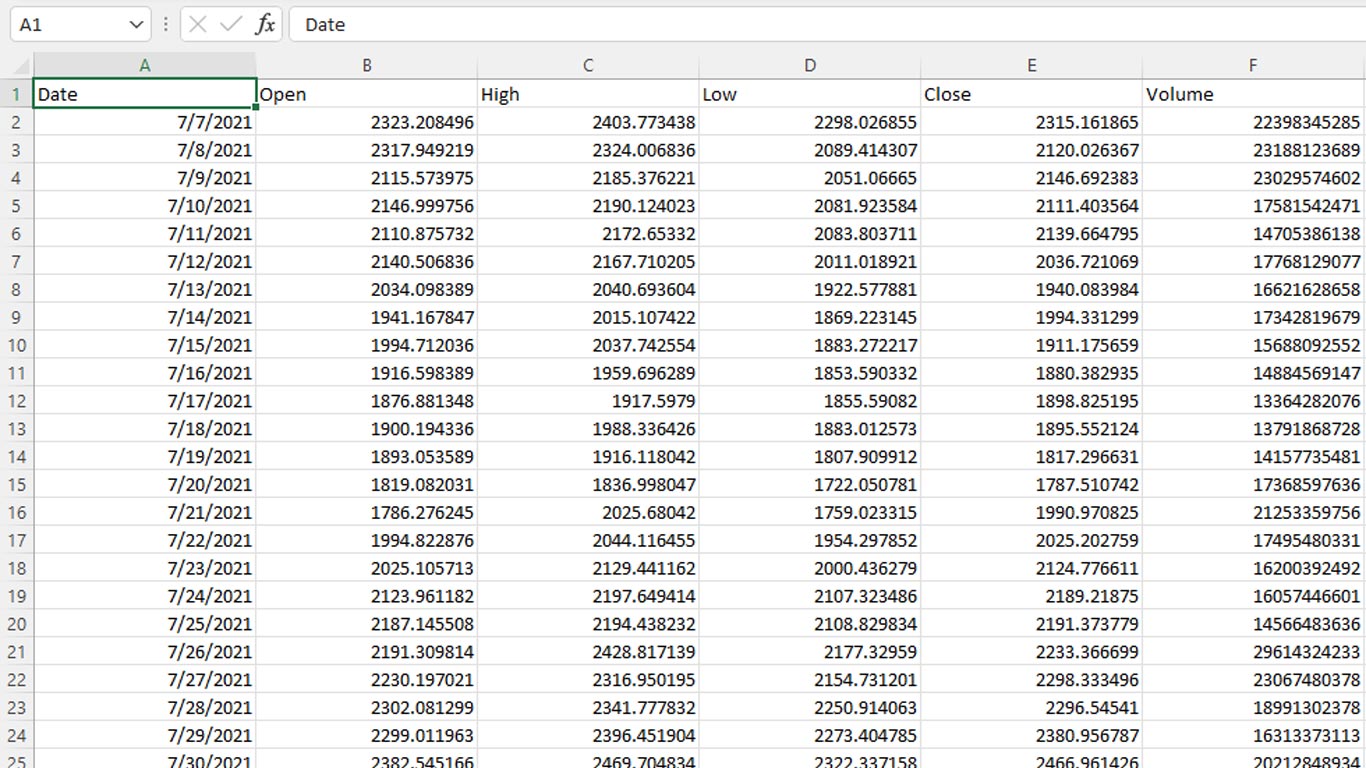
Here we see our data as expected. Now, imagine we had already downloaded this data as a CSV file and needed to load the CSV file as a Pandas DataFrame to perform some analysis. Fortunately, that’s easy as well!
Load A CSV File as DataFrame
We will use our local file saved from before to load back into memory as a DataFrame object. Consider the following example code:
import pandas as pd

# Specify our filename
filename = 'eth-usd-20210707-20220707.csv'

# Load CSV file as DataFrame via the read_csv method
df = pd.read_csv(filename)

# View result
print(df)

           Date         Open  ...        Close       Volume
0    2021-07-07  2323.208496  ...  2315.161865  22398345285
1    2021-07-08  2317.949219  ...  2120.026367  23188123689
2    2021-07-09  2115.573975  ...  2146.692383  23029574602
3    2021-07-10  2146.999756  ...  2111.403564  17581542471
4    2021-07-11  2110.875732  ...  2139.664795  14705386138
..          ...          ...  ...          ...          ...
361  2022-07-03  1066.467407  ...  1073.766968   8557248150
362  2022-07-04  1073.794312  ...  1151.059082  13670889311
363  2022-07-05  1150.509766  ...  1134.541016  16195518291
364  2022-07-06  1134.822266  ...  1186.973999  15373536703
365  2022-07-07  1187.752075  ...  1185.904053  13014859776

[366 rows x 6 columns]
The data has loaded as expected but there is an issue: the Date the column is no longer the first column! We now have an integer-based index for the DataFrame. Fortunately, this can be resolved by explicitly specifying which column the data should be indexed by.
Manually specifying the index column for a DataFrame can be done in one of two ways.
- Via the
index_colargument during import via theread_csvmethod. - Via the
set_indexargument on an existing DataFrame.
Method 1: Specify DataFrame Index During CSV Import
The following code will set the Date column as the DataFrame index during the import of data via the read_csv method:
# Load local CSV file as DataFrame
df = pd.read_csv(filename, index_col='Date')

# view output
print(df)

                   Open         High          Low        Close       Volume
Date
2021-07-07  2323.208496  2403.773438  2298.026855  2315.161865  22398345285
2021-07-08  2317.949219  2324.006836  2089.414307  2120.026367  23188123689
2021-07-09  2115.573975  2185.376221  2051.066650  2146.692383  23029574602
2021-07-10  2146.999756  2190.124023  2081.923584  2111.403564  17581542471
2021-07-11  2110.875732  2172.653320  2083.803711  2139.664795  14705386138
...                 ...          ...          ...          ...          ...
2022-07-03  1066.467407  1083.418945  1044.005615  1073.766968   8557248150
2022-07-04  1073.794312  1152.943848  1048.396362  1151.059082  13670889311
2022-07-05  1150.509766  1165.682739  1086.829956  1134.541016  16195518291
2022-07-06  1134.822266  1193.636719  1116.247559  1186.973999  15373536703
2022-07-07  1187.752075  1187.752075  1165.623169  1185.904053  13014859776

[366 rows x 5 columns]
Method 2: Specify DataFrame Index on Existing DataFrame
A DataFrame can either be reindexed and assigned to a new variable (i.e. a copy) or reindexed in place. Either approach utilizes the set_index method and the results are determined by the use of the inplace keyword argument. Let’s take a look at both approaches.
# Load local CSV file as DataFrame
df = pd.read_csv(filename)

# view initial data
print(df)

           Date         Open  ...        Close       Volume
0    2021-07-07  2323.208496  ...  2315.161865  22398345285
1    2021-07-08  2317.949219  ...  2120.026367  23188123689
2    2021-07-09  2115.573975  ...  2146.692383  23029574602
3    2021-07-10  2146.999756  ...  2111.403564  17581542471
4    2021-07-11  2110.875732  ...  2139.664795  14705386138
..          ...          ...  ...          ...          ...
361  2022-07-03  1066.467407  ...  1073.766968   8557248150
362  2022-07-04  1073.794312  ...  1151.059082  13670889311
363  2022-07-05  1150.509766  ...  1134.541016  16195518291
364  2022-07-06  1134.822266  ...  1186.973999  15373536703
365  2022-07-07  1187.752075  ...  1185.904053  13014859776

[366 rows x 6 columns]

# reindex (Note: doesn't work in place w/o assignment)
df.set_index('Date')

# view result
print(df)
           Date         Open  ...        Close       Volume
0    2021-07-07  2323.208496  ...  2315.161865  22398345285
1    2021-07-08  2317.949219  ...  2120.026367  23188123689
2    2021-07-09  2115.573975  ...  2146.692383  23029574602
3    2021-07-10  2146.999756  ...  2111.403564  17581542471
4    2021-07-11  2110.875732  ...  2139.664795  14705386138
..          ...          ...  ...          ...          ...
361  2022-07-03  1066.467407  ...  1073.766968   8557248150
362  2022-07-04  1073.794312  ...  1151.059082  13670889311
363  2022-07-05  1150.509766  ...  1134.541016  16195518291
364  2022-07-06  1134.822266  ...  1186.973999  15373536703
365  2022-07-07  1187.752075  ...  1185.904053  13014859776

[366 rows x 6 columns]


# make copy
df = df.set_index('Date')

# view result
print(df)

                   Open         High          Low        Close       Volume
Date
2021-07-07  2323.208496  2403.773438  2298.026855  2315.161865  22398345285
2021-07-08  2317.949219  2324.006836  2089.414307  2120.026367  23188123689
2021-07-09  2115.573975  2185.376221  2051.066650  2146.692383  23029574602
2021-07-10  2146.999756  2190.124023  2081.923584  2111.403564  17581542471
2021-07-11  2110.875732  2172.653320  2083.803711  2139.664795  14705386138
...                 ...          ...          ...          ...          ...
2022-07-03  1066.467407  1083.418945  1044.005615  1073.766968   8557248150
2022-07-04  1073.794312  1152.943848  1048.396362  1151.059082  13670889311
2022-07-05  1150.509766  1165.682739  1086.829956  1134.541016  16195518291
2022-07-06  1134.822266  1193.636719  1116.247559  1186.973999  15373536703
2022-07-07  1187.752075  1187.752075  1165.623169  1185.904053  13014859776

[366 rows x 5 columns]
Here we see three things:
- Our data loaded as expected
- Our data was not reindexed after using the
set_indexmethod because we didn’t specify theinplacekeyword OR we didn’t assign the result to a new variable. - Our data reindexed as intended via assignment to the
dfvariable (overwriting previous data)
Now, let’s consider how using the inplace argument can simply things when the original data is no longer needed:
# Load local CSV file as DataFrame
df = pd.read_csv(filename)

# view initial data
print(df)

           Date         Open  ...        Close       Volume
0    2021-07-07  2323.208496  ...  2315.161865  22398345285
1    2021-07-08  2317.949219  ...  2120.026367  23188123689
2    2021-07-09  2115.573975  ...  2146.692383  23029574602
3    2021-07-10  2146.999756  ...  2111.403564  17581542471
4    2021-07-11  2110.875732  ...  2139.664795  14705386138
..          ...          ...  ...          ...          ...
361  2022-07-03  1066.467407  ...  1073.766968   8557248150
362  2022-07-04  1073.794312  ...  1151.059082  13670889311
363  2022-07-05  1150.509766  ...  1134.541016  16195518291
364  2022-07-06  1134.822266  ...  1186.973999  15373536703
365  2022-07-07  1187.752075  ...  1185.904053  13014859776

[366 rows x 6 columns]

# reindex  using in place argument
df.set_index('Date', inplace=True)

# view result
print(df)

                   Open         High          Low        Close       Volume
Date
2021-07-07  2323.208496  2403.773438  2298.026855  2315.161865  22398345285
2021-07-08  2317.949219  2324.006836  2089.414307  2120.026367  23188123689
2021-07-09  2115.573975  2185.376221  2051.066650  2146.692383  23029574602
2021-07-10  2146.999756  2190.124023  2081.923584  2111.403564  17581542471
2021-07-11  2110.875732  2172.653320  2083.803711  2139.664795  14705386138
...                 ...          ...          ...          ...          ...
2022-07-03  1066.467407  1083.418945  1044.005615  1073.766968   8557248150
2022-07-04  1073.794312  1152.943848  1048.396362  1151.059082  13670889311
2022-07-05  1150.509766  1165.682739  1086.829956  1134.541016  16195518291
2022-07-06  1134.822266  1193.636719  1116.247559  1186.973999  15373536703
2022-07-07  1187.752075  1187.752075  1165.623169  1185.904053  13014859776

[366 rows x 5 columns]
Here we see our original data loaded in, again being indexed via row number. However, after using the inplace=True argument, we note the same DataFrame object is then re-indexed using the Date column without assignment to another variable. This is convenient in cases where the initial data format is no longer needed.
Final Thoughts
Pandas is an incredible library, even if its syntax and opinionated approaches can be difficult to understand at first. It is a highly efficient tool for analyzing, manipulating, and — as we’ve seen here — performing I/O operations on CSV files! The ability to conveniently and quickly specify by which column a DataFrame should index one’s data is critical — especially in cases of time series data.
Converting a DataFrame to CSV is essential for supporting data permanence after computationally-heavy tasks. The CSV format is an ideal format that allows structured data to persist without requiring the overhead of a database. Another alternative is JSON, which Pandas can readily load and convert to CSV or a DataFrame as well! Check out our article on linear regression in Python to see how such heavy number crunching can be facilitated by DataFrames.


