The Average Daily Range is a technical indicator used to measure volatility in an asset. It calculates the average difference between the highest and lowest price over a time interval. Typically, this indicator is used to signal a significant change in price action over the short term.
Introduction
The Average Daily Range (ADR) is similar to a moving average in that it reflects the average of previous values. This helps smooth out noise and reflects a better representation of an asset over time. In this guide we’ll cover the following:
- How to calculate the ADR generally
- How to implement an ADR function in Python
- How to apply an ADR function to a DataFrame object in Python
- The downsides of the ADR
- Implementing a modified ADR
- Average Daily Range vs. Average True Range
The ADR can be a great tool in identifying stocks or tradable assets that are currently experiencing high levels of volatility. This can signal an increase in volume, response to events like news, or abrupt changes in price action. Before we dive in, let’s first talk a bit more about what the ADR is conceptually and how it’s used.
What’s the ADR
The ADR is a measure of volatility and is useful to describe whether an assets price action is outside the normal during a particular time. The daily range (highest price – lowest) can be compared to the ADR over a previous interval to signal potential entry and exit points for traders.
The ADR can be used over whatever interval one chooses, though a 20-day period is common. In stock market technical analysis, this period uses the previous 19 values—along with the current value—to calculate an averaged number for the daily trading range. This can help signal abrupt changes in price action and is useful in stock screeners.
Calculating the ADR
The Average Daily Range is calculated similarly to how one calculates a simple moving average. The difference between the Average Daily Range and a simple moving average is that we must pre-calculate the difference between the high and low for each period. After these values are calculated one can calculate the ADR. The average daily range formula is as follows:

Equations can be a bit heady and often confuse otherwise simple calculations. An iterative approach to calculating the ADR is outlined as such:
- Define a “lookback” interval (K)
- For each period, calculate Daily Range (DR) as:
- High – Low to get the Daily Range (Hxi – Lxi)
- Sum all Daily Range values
- Divide by the lookback interval length
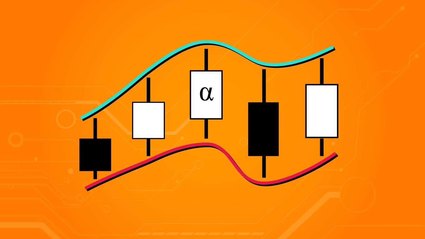
Let’s consider an illustration of the above. First, anyone unfamiliar with candlestick representation of stock prices should check out this article. In the illustration below we can see the Daily Range calculated for each period over a 5-day interval (K) and then added together and divided by K. This gives us the ADR for that period.

This image depicts a stock price that is gradually becoming more volatile over a 5-day period. The first period has a Daily Range of 2 while the last two periods have a daily range of 4. The average daily range here is 3.2 —accounting for the daily range of each period.
Calculating the Average Daily Range in Python
We’ve now seen the mathematical basis for calculating the ADR. Modern trading doesn’t rely on pencil and paper, however. To deploy the ADR as an analytical tool we will implement our logic so far as a Python function. First, let’s create a representation of the price action shown in the image above.
# Five prices as High and Low for the
# five day period K
prices = [
    {"high": 5, "low": 3},
    {"high": 7, "low": 4},
    {"high": 9, "low": 6},
    {"high": 7, "low": 3},
    {"high": 8, "low": 4},
]

# Example access
day_one_high    = prices[0]["high"]
day_one_low     = prices[0]["low"]
In practice, it would be practical to have this type of data stored as OHLCV in a pandas DataFrame object. We’re using a list of 5 dictionary objects here for syntactic clarity. Keeping in mind our algorithm outlined above, we can implement the ADR in Python as follows:
# Create list for Daily Range values
daily_ranges = []

# Get High - Low (DR) for each period
for price in prices:

    # Calculate DR
    pct_daily_range = price["low"] / price["high"]

    # Normalize
    daily_ranges.append(100 * (pct_daily_range - 1))

# Calculate Average Daily Range
average_daily_range = sum(daily_ranges) / len(daily_ranges)

# View output
print(average_daily_range)

>>> 3.2
Here we see our result matches up to the manual calculation from the illustrated process above. The example code above is a bit bloated—mostly for sake of clarity—so we’ll tighten things up a bit before we start looking at more practical examples:
# calculate ADR from list of (high, low) tuples
sum([x[0] - x[1] for x in prices]) / len(prices)
This one-liner will make calculating the ADR for some real-world data a bit less syntactically cumbersome. To showcase the utility of the ADR we will fetch the latest stock pricing data and use the resulting DataFrame object for our ADR calculations.
ADR Example
We are going to use the yfinance library to fetch pricing data for Ether ($ETH-USD) over the past 6 months. We can get this data with the following code:
# Get pricing data
import yfinance as yf

# Get the previous 6 months pricing data for ETH and limit to High, Low
ETH = yf.Ticker('ETH-USD').history(period='6mo', interval="1d")[["High", "Low"]]

# View resulting dataframe
print(ETH)

                   High          Low
Date
2021-05-18  3562.465088  3246.404053
2021-05-19  3437.935791  1952.460205
2021-05-20  2993.145264  2170.229004
2021-05-21  2938.205078  2113.347168
2021-05-22  2483.983154  2168.124268
...                 ...          ...
2021-11-14  4689.842773  4516.935547
2021-11-15  4764.636230  4546.599121
2021-11-16  4891.704590  4144.334961
2021-11-17  4300.306641  4107.125977
2021-11-18  4343.557129  4138.691406

[185 rows x 2 columns]
Here we have queried the Yahoo Finance API (sort of) and retrieved the previous 6-months pricing data for $ETH-USD and removed all data but the High and Low value for each day, while also keeping the date as the index values.
Step 1: Calculate Daily Range Values
For each period in our interval, we need to calculate the daily range from the High – Low calculation. This is done using the apply method of the DataFrame object as such:
# Calculate Daily Range for each period
ETH['dr'] = ETH.apply(lambda x: x["High"] - x["Low"], axis=1)


# Result
                   High          Low           dr
Date
2021-05-18  3562.465088  3246.404053   316.061035
2021-05-19  3437.935791  1952.460205  1485.475586
2021-05-20  2993.145264  2170.229004   822.916260
2021-05-21  2938.205078  2113.347168   824.857910
2021-05-22  2483.983154  2168.124268   315.858887
...                 ...          ...          ...
2021-11-14  4689.842773  4516.935547   172.907227
2021-11-15  4764.636230  4546.599121   218.037109
2021-11-16  4891.704590  4144.334961   747.369629
2021-11-17  4300.306641  4107.125977   193.180664
2021-11-18  4343.557129  4052.962158   290.594971

[185 rows x 3 columns]
We now have a third column reflecting the difference in our daily High and daily Low. Next, we need to calculate the average of these values over a preceding period. To do this—effectively calculating a moving average—we will use the rolling method of the DataFrame.
Step 2: Calculate Average Daily Range
Before we calculate the Average Daily Range we need to define our lookback period. A common value for this is 20 periods and what we will use here. This decision means that every ADR value we calculate is reflective of the previous 19 periods of price action plus the range of the current period. This can be achieved via the following code:
# Add a simple moving average
ETH["adr"] = ETH['dr'].rolling(window=20).mean()

# View result
                   High          Low           dr         adr
Date
2021-05-18  3562.465088  3246.404053   316.061035         NaN
2021-05-19  3437.935791  1952.460205  1485.475586         NaN
2021-05-20  2993.145264  2170.229004   822.916260         NaN
2021-05-21  2938.205078  2113.347168   824.857910         NaN
2021-05-22  2483.983154  2168.124268   315.858887         NaN
...                 ...          ...          ...         ...
2021-11-14  4689.842773  4516.935547   172.907227  217.784058
2021-11-15  4764.636230  4546.599121   218.037109  219.570532
2021-11-16  4891.704590  4144.334961   747.369629  238.494238
2021-11-17  4300.306641  4107.125977   193.180664  228.781030
2021-11-18  4343.557129  4052.962158   290.594971  234.109387

[185 rows x 4 columns]
A few things to note: first, we see a new column has been added for the ADR. Secondly—and most important—we see a value of NaN for the first entries. This is because there are fewer than 19 (20 – 1) preceding values for these dates.
We need a minimum of 20 values to calculate the ADR since that is how we defined our lookback window. For example, if we were to print out rows 18-22 we can see where the transition takes place:
# Print rows # 18-21
print(ETH.iloc[17:21])

                   High          Low          dr         adr
Date
2021-06-04  2857.165527  2562.637451  294.528076         NaN
2021-06-05  2817.484863  2558.233643  259.251221         NaN
2021-06-06  2743.441162  2616.162354  127.278809  435.919141
2021-06-07  2845.185059  2583.995117  261.189941  433.175586
In row #20 for the date 2021-06-06, we have our first DR value where there are enough preceding values to calculate the average using our 20-period lookback window.
Modified ADR
The ADR is a great measure of volatility and can help signal a great opportunity to traders and investors. However, it has the shortcoming of being very specific to the price action of a single stock. For example, the ADR of $ETH-USD during the past several days has been around $220USD.
What happens when we try to compare $ETH-USD‘s ADR to an asset whose price is between $5USD and $10USD? It’s certainly not going to be taking $220 swings! However, the percent change in price would still be comparable.
To use the ADR as a screening tool, such that one can compare volatility among different assets equally, we need to modify the ADR formula to reflect a percentage change rather than a fixed dollar change. For this, we need to adjust our algorithm as follows:
- Define a “lookback” interval (K)
- For each period, calculate Daily Range % (DR) as High / Low
- Sum all Daily Range % values
- Divide by the lookback interval length
- Subtract 1 from the DR%
- Multiply by 100
This gives us an ADR representing a percentage change in price which allows comparison between assets with wildly different prices. The following image reflects the update to our ADR algorithm:

We can implement this modified ADR using the following code (using our initial sample data again):
# Get High/Low for each period
daily_ranges = [d[1] / d[0] for d in data]

# Get SMA of daily Ranges
sma = mean(daily_ranges)

# Calculate
modified_adr = 100 * (sma - 1)

>>> 85.0
Note that, once again, we arrive the same value as illustrated in the image. This is good news—indicating our math is correct—but we’re once again left with a syntactically cumbersome algorithm. Let’s use our $ETH-USD DataFrame and employ a once-again-simplified version of our modified ADR:
# Get pricing data
import yfinance as yf

# Get the previous 6 months pricing data for ETH
ETH = yf.Ticker('ETH-USD').history(period='6mo', interval="1d")[["High", "Low"]]

# Calculate Daily Range for each period and normalize as pct change
ETH['dr_pct'] = ETH.apply(lambda x: 100 * (x["High"] / x["Low"] - 1), axis=1)

# Calculate the average daily range over a 20-period interval
ETH["mod_adr"] = ETH['dr_pct'].rolling(window=20).mean()

# View Result
print(ETH)

                   High          Low     dr_pct   mod_adr
Date
2021-05-18  3562.465088  3246.404053   9.735727       NaN
2021-05-19  3437.935791  1952.460205  76.082246       NaN
2021-05-20  2993.145264  2170.229004  37.918407       NaN
2021-05-21  2938.205078  2113.347168  39.030876       NaN
2021-05-22  2483.983154  2168.124268  14.568302       NaN
...                 ...          ...        ...       ...
2021-11-14  4689.842773  4516.935547   3.827976  5.057539
2021-11-15  4764.636230  4546.599121   4.795609  5.075362
2021-11-16  4891.704590  4144.334961  18.033524  5.507737
2021-11-17  4300.306641  4107.125977   4.703549  5.246916
2021-11-18  4343.557129  3985.766113   8.976719  5.480348

[185 rows x 4 columns]
Looking at the last few rows of data we see a modified ADR value in the range of 5-5.48. This reflects an average daily price range as a percentage movement which, once again, requires the first 19 dr_pct values to have been calculated before the first ADR value will be calculated.
Interpretation
The ADR is a measure of volatility. Traditional ADR values represent dollar changes of an asset and are not comparable to other assets. Conceivably, one could make comparisons of assets with very similar prices.
The modified ADR we’ve discussed here can be used to make observations such as the following:
- Asset XYZ changes 3.5% on an average day;
- Asset XYZ changes 3.5% and asset ABC changes 2.0% therefore XYZ is more volatile;
- The ADR of XYZ has been steadily increasing over the past year indicating a steady increase in volatility;
- After a 60% gain and tremendous volume, asset XYZ has been in a volatility contraction pattern for the bast 8 weeks indicated by an ever-decreasing ADR measure.
Keep in mind the ADR and the modified ADR are but tools to analyze price action. Any trading strategy based solely on their indication isn’t likely to be successful. Remember, this technical indicator is available to all other traders on the market as well.
Using it in conjunction with other technical indicators such as the RSI, Bollinger bands, Mean Average Convergence Divergence (MACD), or simple moving averages can give a much more informed perspective of the movement of an underlying asset in the future.
Average Daily Range (ADR) vs. Average True Range (ATR)
The Average Daily Range reflects the average change in intraday prices over a period of time. The Average True Range is similar but takes into account any gaps in pricing between the closing of one trading period and the opening of the next.
Where ADR uses the High and Low of each period to make a calculation the ATR takes into account the High and Low relative to the previous closing price. This accounts for both gaps up and down in price.
Final Thoughts
The Average Daily Range can be a useful tool in developing a range of trading strategies. For example, one could use it as a feature to develop a linear regression model to help forecast price changes in an underlying asset. As with most technical indicators, the ADR is often used alongside others rather than a single predictive measure.
Also, keep in mind that the ADR doesn’t reflect gaps up and down in price. For longer trading windows the ATR may serve as a better reflection of volatility. The implementation we’ve seen in this guide hasn’t been optimized for wide-scale use and has been presented with